
“As simple as possible, but no simpler.”
—Albert Einstein, 1879–1955, Physicist
As discussed in Chapter 1, the basic principles that apply to the analysis and solution of flow problems include the conservation of mass, energy, and momentum, in addition to appropriate transport relations for these conserved quantities. For flow problems, these conservation laws are applied to a system, which is defined as any clearly specified region or volume of fluid with either macroscopic or microscopic dimensions (this is also sometimes referred to as a “control volume”), as illustrated in Figure 5.1. The material (fluid) within the system is assumed to be a continuum, with physical properties that can be defined at all points within the system. This means that only dimensions which are very large compared to the molecular or particulate structure of the material are considered. The general conservation law is
where X is the conserved quantity, that is, mass, energy, or momentum. In the case of momentum, because a “rate of momentum” is equivalent to a force (by Newton’s second law), the “rate in” term must also include any (net) forces acting on the system. It is emphasized that the system is not the “containing vessel”per se (e.g., a pipe, tank, or pump) but is the fluid contained within the designated boundary. We will show how this generic expression is applied for each of the conserved quantities.
For a given system (e.g., Figure 5.1), each entering stream (i) will carry mass into the system (at rate ṁi) and each exiting stream (o) carries mass out of the system (at rate ṁo). Hence, the conservation of mass, or “continuity,” equation for the system is
(5.1) |
where ms is the mass of the system. For each stream
(5.2) |
where
is the local velocity through area
is the average velocity through the total cross section
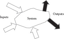
FIGURE 5.1 A system with inputs and outputs.
That is, the total mass flow rate through a given area for any stream is the integrated value of the local mass flow rate over that area. Note that mass flow rate is a scalar, whereas velocity and area are vectors. The scalar (or dot) product of the velocity and area vectors gives the volumetric flow rate which, when multiplied by the density, gives the mass flow rate. The “direction” or orientation of the area is that of the unit vector that is normal to the area and pointing outward from the system. The corresponding definition of the average velocity through the conduit is
(5.3) |
where Q = ṁ/ρ is the volumetric flow rate and the area A is the projected component of that is parallel to , that is, the component of whose normal is in the same direction as .
For a system at steady state, there will be no accumulation of mass in the system, and Equation 5.1 reduces to
(5.4) |
or
(5.5) |
Example 5.1
Water is flowing at a velocity of 7 ft/s in both 1 in. and 2 in. ID pipes, which are joined together and fed into a 3 in. ID pipe, as shown in Figure E5.1. Determine the water velocity in the 3 in. pipe.
Solution:
The system is the fluid within the pipe branch, which is at a steady state so that Equation 5.5 applies:
For a constant density fluid, this may be solved for V3:
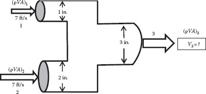
FIGURE E5.1 Application of continuity equation.
Since A = πD2/4, this gives
(Note: The number of significant figures in this problem is indeterminate, so we report the answer to three figures, which is the maximum allowed unless more can be justified.)
The conservation of mass can be applied to an arbitrarily small fluid element (see Figure 5.2) to derive the “microscopic continuity” equation, which must be satisfied at all points within any continuous fluid. This can be done by considering an arbitrary (cubical) differential element of dimensions dx, dy, dz, with mass flow components into or out of each surface, for example,
(5.6) |
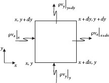
FIGURE 5.2 Two-dimensional microscopic element.
Dividing by the volume of the element (dx dy dz) and taking the limit as the size of the element shrinks to zero gives
(5.7) |
This is the microscopic (local) continuity equation and must be satisfied at all points within any flowing fluid continuum. If the fluid is incompressible (i.e., constant ρ), Equation 5.7 reduces to
(5.8) |
We will make use of this equation later on.
Energy can take a wide variety of forms, such as internal (thermal), mechanical, work, kinetic, potential, surface, electrostatic, electromagnetic, and nuclear energy. Also, for nuclear reactions or velocities approaching the speed of light, the interconversion of mass and energy can be significant. However, we will not be concerned with situations involving nuclear reactions or velocities near that of light, and some other possible forms of energy (such as surface tension) may be negligible as well. Our purpose will be adequately served if we consider only internal (thermal), kinetic, potential (due to gravity and/or pressure), mechanical (work), and thermal (heat) forms of energy. For the system illustrated in Figure 5.1, a unit mass of fluid in each inlet and outlet stream may contain a certain amount of internal energy (u) by virtue of its temperature, kinetic energy (v2/2) by virtue of its velocity, potential energy (gz) due to its position in a (gravitational) potential field, and “pressure (PV/m) or (P/ρ)” energy. The “pressure energy” is sometimes called the “flow work,” because it is associated with the amount of work or energy required to “inject” a unit mass of fluid into the system or “eject” it out of the system at the appropriate pressure. In addition, energy can cross the boundaries of the system other than with the flow streams in the form of heat (Q), resulting from a temperature difference, and “shaft work” (W). Shaft work is so named because it is normally associated with work transmitted to or from the system by a shaft, such as that of a pump, compressor, mixer, or turbine.
The sign convention for heat (Q) and work (W) is arbitrary and consequently varies from one reference to another. Heat is usually taken to be positive when it is added to the system, so it would seem to be consistent to use this same convention for work (which is the convention in most “scientific” references). However, engineers, being “pragmatic,” use a sign convention that is directly associated with “value.” That is, if work can be extracted_from the system (e.g., to drive a turbine), then it is positive, because a positive asset can be sold to produce revenue. However, if work must be put into the system (such as by a pump or a mixer), then it is negative, because the energy must be purchased to drive the pump (a negative asset). This convention is also more consistent with the “driving force” interpretation of the terms in the energy balance, as will be shown later.
With this introduction, we can write the rate form of the conservation of energy equation for any system as follows, in which each term in brackets (…) represents a form of energy per unit of mass of fluid:
(5.9) |
Here, h = u+P/ρ is the enthalpy per unit mass of fluid. Note that the inlet and exit streams include enthalpy (i.e., internal energy, u, plus flow work, P/ρ), whereas the “system energy” includes only the internal energy but no P/ρ flow work (for obvious reasons). If there is only one inlet stream and one exit stream and the system is at steady state (i.e., ṁi = ṁo = ṁ), the energy balance becomes
(5.10) |
where
Δ(…) = (“out”) – (“in”), and
represents the heat added to the system and work done by the system, respectively, per unit mass of fluid
The system may also be composed of the fluid between any two points along a streamline (e.g., a “stream tube”) within a flow field. Specifically, if these two points are only an infinitesimal distance apart, the result is the differential form of the energy balance:
(5.11) |
where dh = du+ d(P/ρ). The “d()” notation represents a total or “exact” differential and applies to those quantities that are determined only by the state (T, P) of the system and are thus “point” properties. The “δ()” notation represents quantities which are inexact differentials and depend upon the path taken from one point to another.
Note that the energy balance contains several different forms of energy, which may be generally classified as either mechanical energy, associated with motion or position, or thermal energy, associated with temperature. Mechanical energy is “useful,” in that it can be converted directly into useful work, and includes potential energy, kinetic energy, “flow work,” and shaft work. The thermal energy terms, that is, internal energy and heat, are not directly available to do useful work unless they are transformed into mechanical energy, in which case it is the mechanical energy that does the useful work.
In fact, the total amount of energy represented by a relatively small temperature change is equivalent to a relatively large amount of “mechanical energy.” For example, 1 Btu of thermal energy is equivalent to 778 ft lbf of mechanical energy. This means that the amount of energy required to raise the temperature of lbm of water by 1°F (the definition of the Btu) is equivalent to the amount of energy required to raise the elevation of that same pound of water by 778 ft (e.g., an 80 story building!). Thus, for systems that involve significant temperature changes, the mechanical energy terms (e.g., pressure, potential and kinetic energy, and work) may be negligible compared with the thermal energy terms (e.g., heat transfer, internal energy). In such cases, the energy balance equation reduces to a “heat balance,” that is, Δh = q. However, the reader should be warned that “heat” is not a conserved quantity and that the inherent assumption that the other forms of energy are negligible when a “heat balance” is being written should always be confirmed.
Before proceeding further, we will take a closer look at the significance of enthalpy and internal energy, because these cannot be measured directly but are determined indirectly by measuring other properties such as temperature and pressure.
An infinitesimal change in internal energy is an exact differential and is a unique function of temperature and pressure (for a given composition). Since the density of a given material is also uniquely determined by temperature and pressure (e.g., by an equation of state for the material), the internal energy may be expressed as a function of any two of the three variables T, P, or ρ (or v = 1/ρ). Hence, we may write
(5.12) |
By making use of classical thermodynamic identities, this is found to be equivalent to
(5.13) |
where
(5.14) |
is the specific heat at constant volume (e.g., constant density). We will now consider several special cases for various materials.
For an ideal gas
(5.15) |
Thus, Equation 5.13 reduces to
(5.16) |
where is the average constant volume heat capacity between the two temperatures T1 and T2. This shows that the internal energy for an ideal gas is a function of temperature only.
For a nonideal gas, Equation 5.15 is not valid, so that
(5.17) |
Consequently, the term in brackets in Equation 5.13 does not cancel out as it did for the ideal gas, which means that, for a non-ideal gas,
(5.18) |
The form of the implied function, fn(T, P), may be analytical if the material is described by a nonideal equation of state or it could be empirical, such as for steam, for which the properties are expressed as data tabulated in steam tables.
For solids and liquids, ρ ≈ constant (or dv = 0), so
(5.19) |
This shows that the internal energy depends upon temperature only (just as for the ideal gas, but for an entirely different reason).
The enthalpy can be expressed as a function of temperature and pressure:
(5.20) |
which, from thermodynamic identities, is equivalent to
(5.21) |
where
(5.22) |
is the specific heat of the material at constant pressure. We again consider some special cases.
For an ideal gas
(5.23) |
Thus, Equation 5.21 for the enthalpy becomes
(5.24) |
which shows that the enthalpy for an ideal gas is a function of temperature only (as is the internal energy).
For a nonideal gas
(5.25) |
which, like Δu, may be either an analytical or an empirical function. All gases follow the ideal gas law under appropriate conditions (i.e., far enough from the critical point) and become more nonideal as the critical point is approached. That is, under conditions that are sufficiently far from the critical point that the enthalpy at constant temperature is essentially independent of pressure, the gas should be adequately described by the ideal gas law. This can be confirmed by inspecting the thermodynamic plots for various materials shown in Appendix D.
For solids and liquids, v = 1/ρ ≈ constant, so that (∂v/∂T)P = 0 and cp≈ cv. Therefore, Equation 5.21 reduces to
(5.26) |
or
(5.27) |
This shows that for solids and liquids, the enthalpy depends upon both temperature and pressure. This is in contrast to the internal energy, which depends upon the temperature only. Note that for solids and liquids, cp ≈ cv.
The thermodynamic properties of a number of compounds are shown in Appendix D as pressure–enthalpy diagrams with lines of constant temperature, entropy, and specific volume. The vapor, liquid, and two-phase regions are clearly evident on these plots. The conditions under which each compound may exhibit ideal gas properties are identified by the region on the plot where the enthalpy is independent of pressure at a given temperature (i.e., the lower the pressure and the higher the temperature relative to the critical point, the more nearly the properties can be described by the ideal gas law).
We have noted that if there is a significant change in temperature, the thermal energy terms (i.e., q and u) may represent much more energy than the mechanical terms (i.e., pressure, potential and kinetic energy, and work). On the other hand, if the temperature difference between the system and its surroundings is very small, the only source of “heat” (thermal energy) is the internal (irreversible) dissipation of mechanical energy into thermal energy or “friction.” The origin of this “friction loss” is the irreversible work required to overcome intermolecular forces when the fluid is in motion, that is, the attractive forces between the “fluid elements,” under dynamic (nonequilibrium) conditions. This can be quantified as follows.
For a system at equilibrium (i.e., in a reversible or “static” state), thermodynamics tells us that
(5.28) |
That is, the total increase in entropy (which is a measure of “disorder” or “irreversibility”) comes from heat transferred across the system boundary (δq). However, a flowing fluid is in a “dynamic” or irreversible state, which consumes “useful” energy (e.g., mechanical energy) and transforms it into “non-useful” thermal energy (e.g., entropy). Because entropy is proportional to the degree of departure from the most stable (equilibrium) conditions, this means that the further the system is from equilibrium (i.e., the faster the flow), the greater the increase in entropy, so for a dynamic (flow) system
(5.29) |
that is,
(5.30) |
where δef represents the “irreversible energy” associated with the departure of the system from equilibrium, which is extracted from mechanical energy and transformed (or “dissipated”) into thermal energy. The farther the system is from equilibrium (e.g., the faster the motion), the greater is this irreversible energy. The origin of this energy (or “extra entropy”) is the mechanical energy that drives the system and is thus converted to ef. This energy ultimately appears as an increase in the temperature of the system (du), heat transferred from the system (δq), and/or expansion energy [Pd(1/ρ)] (if the fluid is compressible). This mechanism of transfer of useful mechanical energy to low-grade (non-useful) thermal energy is referred to as “energy dissipation.” Although ef is often referred to as the “friction loss,” it is evident that this energy is not really lost but is transformed (dissipated) from useful high-level mechanical energy to non-useful low-grade thermal energy. It should be clear that ef must always be positive because energy can be transformed spontaneously only from a higher state (mechanical) to a lower state (thermal) and not in the reverse direction, as a consequence of the second law of thermodynamics.
When Equation 5.30 is introduced into the definition of enthalpy, we get
(5.31) |
Substituting this for the enthalpy in the differential energy balance, Equation 5.11, gives
(5.32) |
This can be integrated along a streamline from the inlet to the outlet of the system to give
(5.33) |
where, from Equation 5.30,
(5.34) |
Equations 5.33 and 5.34 are simply rearrangements of the steady-state total energy balance (Equation 5.10) but in much more useful form. Without the friction loss (ef) term (which includes all of the thermal energy effects), Equation 5.33 represents a mechanical energy balance (although mechanical energy is not a conserved quantity). Equation 5.33 is the engineering Bernoulli equation or simply the Bernoulli equation. Along with Equation 5.34, it accounts for all of the possible thermal and mechanical energy effects of concern to us and is the form of the energy balance that is most convenient when mechanical energy dominates and thermal effects are minor. It should be stressed that the first three terms in Equation 5.32 are point functions, that is, they depend only on conditions at the inlet and outlet of the system, whereas the w and ef terms are path functions, which depend on what is happening to the system between the inlet and outlet points (i.e., these are rate dependent and can be determined either empirically or from an appropriate rate or transport model, as will be shown later).
If the fluid is incompressible (constant density), Equation 5.33 can be written as
(5.35) |
where Φ = P+ ρgz is the potential. For a fluid at rest, ef = V = w = 0, and Equation 5.35 reduces to the basic equation of fluid statics for an incompressible fluid (i.e., Φ = constant), Equation 4.8. For any static fluid, Equation 5.35 reduces to the more general basic equation of fluid statics, Equation 4.6. For gases, if the pressure change is such that the density does not change more than about 30%, the incompressible equation can be applied with reasonable accuracy by assuming the density to be constant at a value equal to the average density in the system (a more general consideration of compressible fluids is given in Chapter 9).
Note that if each term of Equation 5.35 is divided by g, then all terms will have the dimension of length. The result is called the “head” form of the Bernoulli equation, and each term then represents the amount of energy in an equivalent static column of the system fluid. For example, the pressure term becomes the “pressure head, (−ΔP/ρg = HP),” the potential energy term becomes the “static head, (−Δz = Hz),” the kinetic energy term becomes the “velocity head, (ΔV2/2g = Hv),” the friction loss becomes the “head loss, (ef/g = Hf),” and the work term is, typically, the “pump head (work), (─w/g = Hw).”
In the foregoing equations, we assumed that the fluid velocity (V) at a given point in the system (e.g., in a pipe or tube) is the same for all fluid elements at a given cross section in the flow stream. However, this is not true in conduits, because the fluid velocity is zero at a stationary boundary or wall and increases with the distance from the wall. The total rate at which kinetic energy is transported by a auid element moving with local velocity at a mass flow rate dṁ through a differential area is where . Therefore, since the density does not vary over the cross section, the total rate of transport of kinetic energy through the cross section A is
(5.36) |
If the fluid velocity is uniform over the cross section at a value equal to the average velocity V (i.e., “plug flow”), then the rate at which kinetic energy is transported would be
(5.37) |
Therefore, a kinetic energy correction factor, α, can be defined as the ratio of the true rate of kinetic energy transport, relative to that which would occur if the fluid velocity is everywhere equal to the average (plug flow) velocity, for example,
(5.38) |
The Bernoulli equation should therefore include this kinetic energy correction factor, that is,
(5.39) |
As will be shown later, the velocity profile for a Newtonian fluid in fully developed laminar flow in a circular tube is parabolic. When this profile is introduced into Equation 5.38, the result is α = 2. For highly turbulent flow, the profile is much flatter and α ≈ 1.06, although for practical applications it is usually assumed that α = 1 for turbulent flow in a tube.
Example 5.2 Kinetic Energy Correction Factor for Laminar Flow of a Newtonian Fluid
We will show later that the velocity profile for the laminar flow of a Newtonian fluid in fully developed flow in a circular tube of radius R is parabolic. Because the velocity is zero at the wall of the tube and maximum in the center, the equation for the profile is
This can be used to calculate the kinetic energy correction factor from Equation 5.38 as follows. First, we must calculate the average velocity, V, using Equation 5.3 and substitute x=r/R:
This shows that the average velocity is simply one-half of the maximum (centerline) velocity. Thus, replacing V in Equation 5.38 by Vmax/2 and then integrating the cube of the parabolic velocity profile over the tube cross section gives α = 2. (The details of the manipulation are left as an exercise for the reader.)
Example 5.3 Diffuser
A diffuser is a section in a conduit over which the flow area increases gradually from upstream to downstream, as illustrated in Figure E5.2. If the inlet and outlet areas (A1, and A2) are known, and the upstream pressure and velocity (P1, and V1,) are given, we would like to find the downstream pressure and velocity (P2 and V2). If the fluid is incompressible, the continuity equation gives V2:
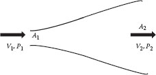
Figure E5.2 Diffuser.
The pressure P2 is determined from the Bernoulli equation. If the diffuser is horizontal, there is no work done between the inlet and outlet, and the friction loss is small (which is a good assumption for a well-designed diffuser), utilizing the continuity (conservation of mass) equation gives
Assuming α1, = α2, the Bernoulli equation gives
Because A1, < A2 and the losses are small, this shows that P2 > P1, that is, the pressure increases downstream as the velocity decreases. This occurs because the decrease in kinetic energy is transformed into an increase in “pressure energy.” Such a diffuser is said to have a “high-pressure recovery.”
Example 5.4 Sudden Expansion
We now consider an incompressible fluid flowing from a small conduit through a sudden expansion into a larger conduit, as illustrated in Figure E5.3. The objective, as in the previous example, is to determine the exit pressure and velocity (P2 and V2), given the upstream conditions and the dimensions of the ducts. Note that the conditions are all identical to those of the previous diffuser example, so the continuity and Bernoulli equations are also identical. The major difference is that the friction loss (a “path” variable) is not small as it is for the diffuser. Because of inertia, the fluid cannot follow the sudden 90° change in direction of the boundary, so considerable secondary flow is generated after the fluid leaves the small duct and before it can expand to fill the large duct, resulting in much greater friction loss. The equation for P2 is the same as before, except that now the friction loss is relatively large (methods for evaluating this will be given later):
The “pressure recovery” is reduced by the friction loss in the eddies which is relatively high for the sudden expansion. The pressure recovery is therefore relatively low and may be negative.
Example 5.5 The Torricelli Problem
Consider an open vessel with diameter D1 containing a fluid at a depth h, that is draining out of a hole of diameter D2 in the bottom of the tank. We would like to determine the velocity of the fluid flowing out of the hole in the bottom. As a first approximation, we neglect the friction loss in the tank and through the hole. Point 1 is taken at the free surface of the fluid in the tank, and point 2 is taken at the exit from the hole, since the pressure is known to be atmospheric at both points (Figure E5.4). The velocity in the tank is related to that through the hole by the continuity equation, with ρ2 = ρ1:
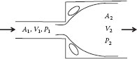
Figure E5.3 Sudden expansion.
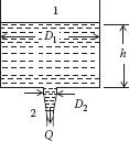
Figure E5.4 Draining tank—the Torricelli problem.
where β = D2/D1. The Bernoulli equation for an incompressible fluid between points 1 and 2 is
Because points 1 and 2 are both at atmospheric pressure, P2 = P1. We assume that w = 0, α = 1, and we neglect friction, so ef = 0 (actually a poor assumption in many cases). Setting (z2 − z1) = −h, eliminating V1 from these two equations, and solving for V2 gives
This is known as the Torricelli equation. We now consider what happens as the hole gets larger. Specifically, as D2 → D1 (i.e., as β → 1), the equation says that V2 → ∞! This is obviously an unrealistic limit, so there must be something wrong. Of course, our assumption that friction is negligible may be valid at low velocities, but as the velocity increases it becomes less valid and is obviously invalid long before the limiting condition is reached.
Upon examining the equation for V2, we see that it is independent of the properties of the fluid in the tank. We might suspect that this is not accurate, because if the tank were to be filled with CO2 we intuitively expect that it would drain more slowly than if it were filled with water. So, what is wrong? In this case, it is our assumption that P2 = P1. Of course, the pressure is atmospheric at both points 1 and 2, but we have neglected the static head of air between these points, which is the actual difference in the pressure. This results in a buoyant force due to the air and can have a significant effect on the drainage of CO2 although it will be negligible for water. Thus, if we account for the static head of air, that is, P2 − P1 = ρagh, in the Bernoulli equation and then solve for V2, we get
where ρ is the density of the fluid in the tank. This also shows that as ρ → ρa, the velocity goes to zero, as we would expect.
These examples illustrate the importance of knowing what can and cannot be neglected in a given problem (i.e., the “baby vs. the bathwater”), and the necessity for matching the appropriate assumptions to the specific problem conditions in order to arrive at a valid solution. They also illustrate the importance of understanding what is happening within the system in addition to knowing the inlet and outlet conditions.
V. CONSERVATION OF LINEAR MOMENTUM
A macroscopic momentum balance for a flow system must include all equivalent forms of momentum. In addition to the rate of linear momentum convected into and out of the system by the entering and leaving streams, the sum of all the forces that act on the system (the system being defined as a specified volume of fluid) must be included. This follows from Newton’s second law, which provides an equivalence between force and the rate of change (and rate of transport) of linear momentum. The resulting macroscopic conservation of linear momentum thus becomes
(5.40) |
Note that because momentum is a vector, this equation represents three component equations, one for each direction in three-dimensional space. If there is only one “in” (entering) and one “out” (leaving) stream, and the system is also at steady state, then ṁi = ṁo = ṁ and the momentum balance becomes
(5.41) |
Note that the vector (directional) character of the “convected” momentum terms (i.e., ) is that of the velocity, because ṁ is a scalar (i.e., is a scalar product).
A. ONE-DIMENSIONAL FLOW IN A TUBE
We will apply the steady-state momentum balance to a fluid in plug flow (i.e., uniform velocity across the cross section) in a tube, as illustrated in Figure 5.3. (The “stream tube” may be bounded by either solid or imaginary boundaries; the only condition is that no fluid crosses the boundaries other than that through the “inlet” and “outlet” planes.)
The shape of the cross section does not have to be circular; it can be any shape. The fluid element in the “slice” of thickness dx is our system, and the momentum balance equation on this system is
(5.42) |
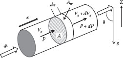
FIGURE 5.3 Momentum balance on a “slice” in a stream tube.
The forces acting on the fluid result from pressure (dFP), gravity (dFg), wall drag (dFw), and external “shaft” work, that is, pump work (δW = −Fext dx, not shown in Figure 5.3):
(5.43) |
where
Here, τw is the stress exerted by the fluid on the wall (the reaction to the stress exerted on the fluid by the wall), and Wp is the perimeter of the cross section that is wetted by the fluid (the “wetted perimeter”). After substituting the expressions for the forces from Equation 5.43 into the momentum balance equation, Equation 5.42, and dividing the result by ─ρA, where A = Ax, the result is
(5.44) |
where δw = δW/(ρA dx) is the work done by the system per unit mass of fluid. Integrating this expression from the inlet (i) to the outlet (o) and assuming steady state gives
(5.45) |
Comparing this with the Bernoulli equation (Equation 5.33) shows that they are identical provided
(5.46) |
or, for steady flow in a uniform conduit,
(5.47) |
where
(5.48) |
is called the hydraulic diameter. Note that this result applies to a conduit of any cross-sectional shape. For a circular tube, for example, Dh is identical to the tube diameter D.
We see that there are several ways of interpreting the term ef. From the Bernoulli equation, it represents the “lost” (i.e., dissipated) energy associated with irreversible effects. From the momentum balance, ef is also seen to be directly related to the stress between the fluid and the tube wall (τw), that is, it can be interpreted as the work required to overcome the resistance to flow in the conduit. Both of these interpretations are correct and are equivalent.
Although the energy and momentum balances lead to equivalent results for this special case of one-dimensional fully developed flow in a straight uniform tube, this is an exception and not the rule. In general, because momentum is a vector, the momentum balance gives additional information concerning the forces exerted on and/or by the fluid in the system through the boundaries, which is not given by the energy balance or Bernoulli equation. This will be illustrated shortly.
Looking at the Bernoulli equation, we see that the friction loss (ef) can be made dimensionless by dividing it by the kinetic energy per unit mass of fluid. The result is the dimensionless loss coefficient, Kf:
(5.49) |
A loss coefficient may be defined for any element that offers resistance to flow (i.e., in which energy is dissipated), such as a length of conduit, a valve, a pipe fitting, a bend, a contraction, or an expansion. The total friction loss can thus be expressed in terms of the sum of the losses in each element, that is, . This will be elaborated in Chapter 6.
As can be determined from Equations 5.47 and 5.49, the pipe wall stress can also be made dimensionless by dividing by the kinetic energy per unit volume of fluid. The result is known as the pipe Fanning friction factor, f:
(5.50) |
Although ρV2/2 represents kinetic energy per unit volume, ρV2 is also the magnitude of the flux of momentum carried by the fluid along the conduit. The latter interpretation is more logical in Equation 5.50, because τw is also a flux of momentum from the fluid to the tube wall. This interpretation renders the factor of ½ arbitrary, although it is related to the kinetic energy of the fluid. Other definitions of the pipe friction factor are also in use, that are some multiple of two times the Fanning friction factor. For example, the Darcy friction factor, which is equal to 4f is used frequently by mechanical and civil engineers. Thus, it is important to know which definition is used or implied when data or charts for friction factors are used.
Because the friction loss and wall stress are related by Equation 5.47, the loss coefficient for pipe flow is related to the pipe Fanning friction factor as follows:
(5.51) |
Example 5.6 Friction Loss in a Sudden Expansion
Figure E5.5 shows the flow in a sudden expansion from a small conduit to a larger one. We assume that the conditions upstream of the expansion (point 1) are known, as well as the areas A1 and A2. We desire to find the velocity and pressure downstream of the expansion (V2 and P2), and the loss coefficient, Kf. As before, V2 is determined from the mass balance (continuity equation) applied to the system (which is all of the fluid in the conduit between points 1 and 2). Assuming a constant density fluid
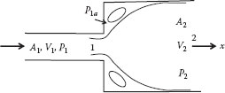
Figure E5.5 Loss coefficient for a sudden expansion.
For plug flow, the Bernoulli equation for this system is
which contains two unknowns, P2 and ef. So, we need another equation, which is the steady-state x component of the momentum balance:
where V1x = V1, and V2x = V2, because all velocities of interest are in the x direction. Accounting for all the forces that can act on the system through each section of the boundary, this becomes
where
P1a is the pressure on the left-hand boundary of the system (i.e., the “washer shaped” surface)
Fwall is the force due to the drag of the wall on the fluid at the horizontal boundary of the system
The fluid pressure cannot change discontinuously, so P1a ≈ P1. Also, because the contact area with the wall bounding the system is relatively small, we can neglect Fwall with no serious consequences. The result is
This can be solved for P2 − P1, which, when inserted into the Bernoulli equation, allows us to solve for ef:
Thus,
The loss coefficient is seen to be a function only of the geometry of the system (note that the assumption of plug flow implies that the flow is highly turbulent). For most systems (i.e., flow in valves, fittings, etc.), the loss coefficient cannot be determined accurately from simple theoretical concepts such as this, but must be determined experimentally. For example, the friction loss in a sudden contraction cannot be calculated by this simple method due to the occurrence of the vena contracta just downstream of the contraction (see Table 7.5 and the discussion in Section IV of Chapter 10). For a sharp 90° contraction, the contraction loss coefficient is given by
where β is the ratio of the small to the large tube diameters.
Example 5.7 Flange Forces on a Pipe Bend
Consider an incompressible fluid flowing through a pipe bend, as illustrated in Figure E5.6. We would like to determine the forces in the bolts in the flanges that hold the bend in the pipe, knowing the geometry of the bend, the flow rate through the bend, and the exit pressure (P2) from the bend. The system is the fluid within the pipe bend, and a steady-state “x momentum” balance on this system is
Various factors contribute to the forces on the left-hand side of this equation, that is,
Since “action = reaction,” the force exerted on the fluid by the solid wall is the negative of the force exerted by the fluid on the wall. This force is then transmitted to the bolts and supports holding the bend in place. The sign of the force resulting from the pressure acting on the inlet and outlet areas is intuitive, because pressure acts on any system boundary from the outside, that is, since the pressure at any point acts equally in all directions, the pressure on the left-hand boundary acts to the right on the system and vice versa. This is also consistent with previous definitions, because the sign of a surface element corresponds to the direction of the normal vector that points outward from the bounded volume, and pressure is a compressive (negative) stress. Thus, P1 Ax1 is (+) since it is a negative stress acting on a negative area, and P2Ax2 is (-) because it is a negative stress acting on a positive area. These signs have been accounted for intuitively in the equation.
The right-hand side of the momentum balance reduces to
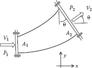
Figure E5.6 Flange forces in a pipe bend.
Equating the expressions for the RHS and LHS of the momentum equation and solving for (Fx)on wall gives
Similarly, the “y momentum” balance is
which becomes
This assumes that the x–y plane is horizontal. If the y direction is vertical, the total weight of the bend, including the fluid inside, could be included as an additional (negative y) force component due to gravity. The magnitude and direction of the net force are
where φ is the direction of the net force vector measured counterclockwise from the +x direction. Note that either P1 or P2 must be known, and the other is determined by the energy balance (Bernoulli equation), assuming that the loss coefficient, Kf, is known:
Methods for evaluating the loss coefficient Kf will be discussed in Chapter 6.
It should be noted that in evaluating the forces acting on the system, the effect of the external pressure transmitted through the boundaries to the system from the surrounding atmosphere was not included. Although this pressure does result in forces that act on the system, these forces all cancel out, so that the pressure that appears in the momentum balance equation is the net pressure in excess of atmospheric, that is, the gage pressure.
C. CONSERVATION OF ANGULAR MOMENTUM
In addition to linear momentum, angular momentum (or the moment of momentum) may be conserved. For a fixed mass (m) moving in the x direction with a velocity of Vx, the linear x momentum (Mx) is mVx. Likewise, a mass (m) rotating counterclockwise about a center of rotation at an angular velocity ω = dθ/dt has an angular momentum (Lθ) equal to mVθR = mωR2, where R is the distance from the center of rotation to the center of the mass m. Note that the angular momentum has dimensions of length times momentum and is therefore also referred to as the “moment of momentum.” If the mass is not a point mass but a rigid distributed mass (M) rotating at a uniform angular velocity, the total angular momentum is given by
(5.52) |
where I is the moment of inertia of the body with respect to the center of rotation.
For a given mass, the conservation of linear momentum is equivalent to Newton’s second law:
(5.53) |
The corresponding expression for the conservation of angular momentum is
(5.54) |
where
Γθ is the moment (torque) acting on the system
dω/dt = α is the angular acceleration
Note the similarity between Equations 5.53 and 5.54. For a flow system, streams with curved streamlines may carry angular momentum into and/or out of the system by convection. To account for this, the general macroscopic angular momentum balance applies:
(5.55) |
For a steady-state system, with only one inlet and one outlet stream, this becomes
(5.56) |
This is also known as the Euler turbine equation, because it applies directly to turbines and all rotating fluid machinery. We will find it useful later in the analysis of the performance of centrifugal pumps.
D. MOVING BOUNDARY SYSTEMS AND RELATIVE MOTION
We sometimes encounter a system that is in contact with a moving boundary, such that the fluid that comprises the system is carried along with the boundary while streams carrying momentum and/or energy may flow into and/or out of the system. Examples of this include the flow impinging on a turbine blade (with the system being the fluid in contact with the moving blade) and the flow of exhaust gases from a moving rocket motor. In such cases, we often have direct information concerning the velocity of the fluid relative to the moving boundary (i.e., relative to the system), Vr, and so we must also consider the velocity of the system, Vs, to determine the absolute velocity of the fluid that is required for the conservation equations.
For example, consider a system that is moving in the x direction with a velocity of Vs, a fluid stream entering the system with a velocity in the x direction relative to the system of Vri, and a stream which leaves the system with a velocity of Vro relative to the system. The absolute stream velocity in the x direction Vx is related to the relative velocity Vrx and the system velocity Vsx by
(5.57) |
and the linear momentum balance equation becomes
(5.58) |
Example 5.8 Turbine Blade
Consider a fluid stream impinging on a turbine blade that is moving with a velocity Vs as shown in Figure E5.7. We would like to know what the velocity of the impinging stream should be in order to transfer the maximum amount of energy to the blade.
The system is the fluid in contact with the blade, which is moving at a velocity Vs. The impinging stream velocity is Vi and the stream leaves the blade at velocity Vo. Since Vo = Vro + Vs and Vi = Vri+ Vs′, the system velocity cancels out of the momentum equation:
If the friction loss is negligible, the energy balance (Bernoulli equation) becomes
which shows that the maximum energy or work transferred from the fluid to the blade occurs when Vo = 0 or Vro = −Vs. Now from continuity at steady state, recognizing that Vi and Vo are of opposite sign
that is,
Rearranging this for Vs gives
Since the maximum energy is transferred when Vo = 0, this reduces to
That is, the maximum efficiency for energy transfer from the fluid to the blade occurs when the velocity of the impinging fluid is twice that of the moving blade (Figure E5.7).
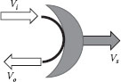
FIGURE E5.7 Turbine blade.
E. MICROSCOPIC MOMENTUM BALANCE
The conservation of momentum principle can be applied to a system composed of the fluid within an arbitrarily small (differential) cubical volume within any flow field. This is done by accounting for convection of mass and momentum through all six surfaces of the cube, all possible stress components acting on each of the six surfaces, and any body forces (e.g., gravity) acting on the mass as a whole. Dividing the result by the volume of the cube and taking the limit as the volume shrinks to zero results in a general microscopic form of the momentum equation that is valid at all points within any fluid. This is done in a manner similar to the earlier derivation of the microscopic mass balance (continuity) equation, Equation 5.7, for each of the three vector components of momentum (see, e.g., Darby, 1976, or many other references). The result can be expressed in general vector notation as
(5.59) |
The three components of this momentum equation, expressed in Cartesian, cylindrical, and spherical coordinates, are given in detail in Appendix E. Note that Equation 5.59 is simply a microscopic (“local”) expression of the conservation of momentum, for example, Equation 5.40, and it applies locally at all points in flowing continuous media.
Note that there are 11 dependent variables, or “unknowns” in these equations , all of which may depend on space and time. (For an incompressible fluid, ρ is constant so there are only 10 “unknowns.”) There are four conservation equations involving these unknowns: the three momentum equations plus the conservation of mass or continuity equation, also given in component form in Appendix E. This means that we still need six more equations (seven, if the fluid is compressible, as the density is also unknown in this case). These additional equations are the “constitutive” equations that relate the local stress components to the rate of deformation of the particular fluid in laminar flow (as determined by the “constitution” or structure of the material), or equations for the local turbulent stress components (the “Reynolds stresses”; see Chapter 6). These equations describe the deformation or flow properties of the specific fluid of interest and relate the six stress components (τij) to the deformation rate (i.e., the velocity gradient components). Note there are only six independent components of the shear stress tensor (τij) because it is symmetrical, i.e., τij· = τij, which is a result of the conservation of angular momentum. For a compressible fluid, the density is related to the pressure through an appropriate “constitutive” equation of state. When the equations for the six τij components are coupled with the four conservation equations, the result is a set of differential equations for the 10 (or 11) unknowns that can be solved (in principle) with appropriate boundary conditions for the velocity components and pressure as a function of time and space for a given flow configuration. In laminar flows, the constitutive equation gives the stress components as a unique function of the velocity gradient components. For example, the constitutive equation for a Newtonian fluid, generalized from the one-dimensional form (i.e., ), is
(5.60) |
where represents the transpose of the matrix of the components. The component forms of this equation are also given in Appendix E for Cartesian, cylindrical, and spherical coordinate systems. If these equations are used to eliminate the stress components from the momentum equations, the result is called the Navier–Stokes equations, which apply to the laminar flow of any Newtonian fluid in any system and are the starting point for the detailed solution of many fluid flow problems. Similar equations can be developed for non-Newtonian fluids, based upon the appropriate rheological (constitutive) model for the fluid (similar to Equation 5.60). For turbulent flows, additional equations are required to describe the momentum transported by the fluctuating (“eddy”) components of the flow (see Chapter 6). However, the number of flow problems for which closed form analytical solutions are possible is rather limited, so numerical (computational) techniques are required for many problems of practical interest. These procedures are beyond the scope of this book, but we will illustrate the application of the continuity and momentum equations to the solution of an example problem.
Example 5.9 Flow Down an Inclined Plane
Consider the steady laminar flow of a thin layer or film of a liquid down a flat plate that is inclined at an angle θ to the vertical, as illustrated in Figure E5.8. The width of the plate is W (normal to the plane of the figure). For convenience, we take the x coordinate direction parallel to the plate in the flow direction, and the y-axis normal to the x-axis, measured from the fluid surface toward the plate. Flow is only in the x direction (parallel to the plane surface), and the velocity varies only in the y direction (normal to the surface). These prescribed conditions, along with the properties of the fluid, constitute the definition of the problem to be solved. The objective is to determine the film thickness, δ, as a function of the flow rate per unit width of plate (Q/W), the fluid properties (μ, ρ), and other parameters in the problem. Since in this case, vy = vz = 0 and the density is constant, the microscopic mass balance (continuity equation) from Appendix E reduces to
This tells us that the velocity vx must be independent of x. Hence, the only independent variable is y. Considering the x component of the momentum equation (see Appendix E), and discarding all y and z velocity and stress components and all derivatives except those with respect to the y direction, the result is
The pressure gradient term has been discarded, because the system is open to the atmosphere and thus the pressure is constant (or, at most, hydrostatic) everywhere (the proof of this is left as an exercise for the reader). This equation can be integrated to give the shear stress distribution in the film:
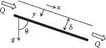
FIGURE E5.8 Flow down an inclined plane.
where the constant of integration is zero, because the shear stress is zero (negligible) at the free surface of the film (y = 0). Note that this result so far is valid for any fluid (Newtonian or non- Newtonian) under any flow conditions (laminar or turbulent), because it is simply a statement of the conservation of mass and momentum. If the fluid is Newtonian and the flow is laminar, the shear stress is
Eliminating the stress between the last two equations gives a differential equation for vx(y) that can be integrated to give the velocity distribution
where the boundary condition that vx = 0 at y = δ (the wall) has been used to evaluate the constant of integration.
The volumetric flow rate can now be determined from
The film thickness (δ) is seen to be proportional to the cube root of the fluid viscosity and the flow rate. The shear stress exerted on the plate is
which is just the component of the weight of the fluid on the plate acting parallel to the plate.
It is also informative to express these results in dimensionless form, that is, in terms of appropriate dimensionless groups. Because this is a “noncircular conduit,” the appropriate flow “length” parameter is the hydraulic diameter, defined by Equation 5.48:
where A is the cross-sectional area of the fluid stream perpendicular to the flow direction and the “wetted perimeter” is simply the width of the plate.
The appropriate form for the Reynolds number is thus
because V = Q/A = Q/(Wδ). The wall stress can also be expressed in terms of the (Fanning) friction factor (Equation 5.50):
Substituting V = Q/Wδ and eliminating ρg cos θ from the expression for Q gives
or
that is, fNRe = 24 = constant. This can be compared with the results of the dimensional analysis for the laminar flow of a Newtonian fluid in a pipe (Section V of Chapter 2), for which we deduced that fNRe = constant. In this case, we have determined the value of the constant analytically using first principles rather than by experiment.
The foregoing procedure can be used to solve a variety of steady, fully developed laminar flow problems, such as flow in a tube, in a concentric annulus, or in a slit between parallel walls, for Newtonian or non-Newtonian fluids. However, if the flow is turbulent, the turbulent eddies transport momentum in three dimensions within the flow field. These contribute additional momentum flux components to the shear stress terms in the momentum equation that must be accounted for. The resulting equations cannot be solved exactly for such flows, and empirical and semiempirical methods for treating turbulent flows will be discussed in Chapter 6.
The key concepts that should be retained from this chapter include:
• The concept of a “system,” comprising a defined volume of fluid on which a balance of conserved quantities can be written.
• The difference between a macroscopic and microscopic balance and the application of each.
• The similarities and differences between the balances of mass, energy, and momentum and the general equations for each.
• The similarities and differences between internal energy and enthalpy for ideal gases and nonideal gases and solids and liquids.
• Irreversible effects in the general Bernoulli equation.
• Conservation of energy and momentum in a straight uniform circular pipe at steady state.
• Definitions of the loss coefficient and friction factor.
• Application of the conservation of momentum to multidimensional systems.
• The conservation of angular momentum.
CONSERVATION OF MASS AND ENERGY
1. Water is flowing into the top of a tank at a rate of 200 gpm. The tank is 18 in. in diameter and has a 3 in. diameter hole in the bottom, through which the water flows out. If the inflow rate is adjusted to match the outflow rate, what will the height of the water be in the tank if friction is negligible?
2. A vacuum pump operates at a constant volumetric flow rate of 10 L/min, evaluated at the pump inlet conditions. How long will it take to pump down a 100 L tank containing air from 1 to 0.01 atm, assuming that the temperature is constant?
3. Air is flowing at a constant mass flow rate into a tank that has a volume of 3 ft3. The temperature of both the tank and the air is constant at 70°F. If the pressure in the tank is observed to increase at a rate of 5 psi/min, what is the mass flow rate of air into the tank?
4. A tank contains water initially at a depth of 3 ft. The water flows out of a hole in the bottom of the tank, and air at a constant pressure of 10 psig is admitted to the top of the tank. If the water flow rate is directly proportional to the square root of the gage pressure inside the bottom of the tank, derive expressions for the water mass flow rate and air mass flow rate as a function of time. Be sure to define all symbols you use in your equations.
5. The flow rate of a hot coal/oil slurry in a pipeline is measured by injecting a small side stream of cool oil and measuring the resulting temperature change downstream in the pipeline. The slurry is initially at 300°F and has a density of 1.2 g/cm3 and a specific heat of 0.7 Btu/(lbm°F). With no side stream injected, the temperature downstream of the mixing point is 298°F. With a side stream at 60°F and a flow rate of 1 lbm/s, the temperature at this point is 295°F. The side stream has a density of 0.8 g/cm3 and a cp of 0.6 Btu/(lbm°F). What is the mass flow rate of the slurry?
6. A gas enters a horizontal 3 in. schedule 40 pipe at a constant rate of 0.5 lbm/s, with a temperature of 70°F and a pressure of 1.15 atm. The pipe is wrapped with a 20 kW heating coil, covered with a thick layer of insulation. At the point where the gas is discharged, the pressure is 1.05 atm. What is the gas temperature at the discharge point, assuming it to be ideal with a MW of 29 and a cp of 0.24 Btu/(lbm°F)?
7. Water is flowing into the top of an open cylindrical tank (diameter D) at a volume flow rate of Qi and out of a hole in the bottom at a rate of Qo. The tank is made of wood that is very porous, and the water is leaking out through the wall uniformly at a rate of q per unit of wetted surface area. The initial depth of water in the tank is z1. Derive an equation for the depth of water in the tank as a function of time. If Qi = 10 gpm, Qo = 5 gpm, D = 5 ft, q = 0.1 gpm/ft2, and z1 = 3 ft, is the level in the tank rising or falling?
8. Air is flowing steadily through a horizontal tube at a constant temperature of 32°C and a mass flow rate of 1 kg/s. At one point upstream where the tube diameter is 50 mm the pressure is 345 kPa. At another point downstream, the diameter is 75 mm and the pressure is 359 kPa. What is the value of the friction loss (ef) between these two points? [cp = 1005 J/(kg K)].
9. Steam is flowing through a horizontal nozzle. At the inlet the velocity is 1000 ft/s and the enthalpy is 1320 Btu/lbm. At the outlet the enthalpy is 1200 Btu/lbm. If heat is lost through the nozzle at a rate of 5 Btu/lbm of steam, what is the outlet velocity?
10. Oil is being pumped from a large storage tank, where the temperature is 70°F, through a 6 in. ID pipeline. The oil level in the tank is 30 ft above the pipe exit. If a 25 hp pump is required to pump the oil at a rate of 600 gpm through the pipeline, what would the temperature of the oil at the exit be, if no heat is transferred across the pipe wall? State any assumptions that you make. Oil properties: SG = 0.92, μ = 35 cp, cp = 0.5 Btu/(lbm°F).
11. Ethylene enters a 1 in. schedule 80 pipe at 170°F and 100 psia and a velocity of 10 ft/s. At a point somewhere downstream, the temperature has dropped to 140°F and the pressure to 15 psia. Calculate the velocity at the downstream conditions and the Reynolds number at both the upstream and downstream conditions.
12. Number 3 fuel oil (30° API) is transferred from a storage tank at 60°F to a feed tank in a power plant at a rate of 2000 bbl/day. Both tanks are open to the atmosphere and are connected by a pipeline containing 1200 ft equivalent length of 1½ in. sch 40 steel pipe and fittings. The level in the feed tank is 20 ft higher than that in the storage tank, and the transfer pump is 60% efficient. The Fanning friction factor is given by
(a) What horsepower motor is required to drive the pump?
(b) If the specific heat of the oil is 0.5 Btu/(lbm°F) and the pump and transfer line are perfectly insulated, what is the temperature of the oil entering the feed tank?
13. Oil with a viscosity of 35 cP, SG of 0.9, and a specific heat of 0.5 Btu/(lbm°F) is flowing through a straight pipe at a rate of 100 gpm. The pipe is 1 in. sch 40, 100 ft long, and the Fanning friction factor is given by . If the temperature of the oil entering the pipe is 150°F, determine
(a) The Reynolds number
(b) The pressure drop in the pipe, assuming that it is horizontal
(c) The temperature of the oil at the end of the pipe, assuming the pipe to be perfectly insulated
(d) The rate at which heat must be removed from the oil (in Btu/h) to maintain it at a constant temperature if there is no insulation on the pipe
14. Water is pumped at a rate of 90 gpm by a centrifugal pump driven by a 10 hp motor. The water enters the pump through a 3 in. sch 40 pipe at 60°F and 10 psig and leaves through a 2 in. sch 40 pipe at 100 psig. If the water gains 0.1 Btu/lbm while passing through the pump, what is the water temperature leaving the pump?
15. A pump driven by a 7.5 hp motor takes water in at 75°F and 5 psig and discharges it at 60 psig at a flow rate of 600 lbm/min. If no heat is transferred to or from the water while it is in the pump, what will the temperature of the water be leaving the pump?
16. A high-pressure pump takes water in at 70°F, 1 atm, through a 1 in. ID suction line and discharges it at 1000 psig through a 1/8 in. ID line. The pump is driven by a 20 hp motor and is 65% efficient. If the flow rate is 500 g/s and the temperature of the discharge is 73°F, how much heat is transferred between the pump casing and the water per pound of water? Does the heat go into or out of the water?
THE BERNOULLI EQUATION
17. Water is contained in two closed tanks (A and B) which are connected by a pipe. The pressure in tank A is 5 psig and that in tank B is 20 psig, and the water level in tank A is 40 ft above that in tank B. Which direction does the water flow?
18. A pump that is driven by a 7.5 hp motor takes water in at 75°F and 5 psig and discharges it at 60 psig at a flow rate of 600 lbm/min. If no heat is transferred between the water in the pump and the surroundings, what will be the temperature of the water leaving the pump?
19. A 90% efficient pump driven by a 50 hp motor is used to transfer water at 70°F from a cooling pond to a heat exchanger through a 6 in. sch 40 pipeline. The heat exchanger is located 25 ft above the level of the cooling pond, and the water pressure at the discharge end of the pipeline is 40 psig. With all valves in the line wide open, the water flow rate is 650 gpm. What is the rate of energy dissipation (friction loss) in the pipeline in kilowatts (kW)?
20. A pump takes water from the bottom of a large tank where the pressure is 50 psig and delivers it through a hose to a nozzle that is 50 ft above the bottom of the tank, at a rate of 100 lbm/s. The water exits the nozzle into the atmosphere at a velocity of 70 ft/s. If a 10 hp motor is required to drive the pump which is 75% efficient, find
(a) The friction loss in the pump
(b) The friction loss in the rest of the system
Express your answer in units of ft lbf/lbm and Nm/kg.
21. You have purchased a centrifugal pump to transport water at a maximum rate of 1000 gpm from one reservoir to another through an 8 in. sch 40 pipeline. The total pressure drop through the pipeline is 50 psi. If the pump has an efficiency of 65% at maximum flow conditions and there is no heat transferred across the pipe wall or the pump casing, calculate
(a) The temperature change of the water through the pump
(b) The horsepower of the motor that would be required to drive the pump
22. The hydraulic turbines at Boulder dam power plant are rated at 86,000 kW when water is supplied at a rate of 66.3 m3/s. The water enters at a head of 145 m at 20°C and leaves through a 6 m diameter duct.
(a) Determine the efficiency of the turbines.
(b) What would be the rating of these turbines if the dam power plant was on Jupiter (g = 26 m/s2)?
23. Water is draining from an open conical funnel at the same rate at which it is entering the top. The diameter of the funnel is 1 cm at the top and is 0.5 cm at the bottom, and it is 5 cm high. The friction loss in the funnel per unit mass of fluid is given by 0.4V2, where V is the velocity leaving the funnel. What is (a) the volumetric flow rate of the water and (b) the value of the Reynolds number entering and leaving the funnel?
24. Water is being transferred by a pump between two open tanks (from A to B) at a rate of 100 gpm. The pump receives the water from the bottom of tank A through a 3 in. sch 40 pipe and discharges it into the top of tank B through a 2 in. sch 40 pipe. The point of discharge into B is 75 ft higher than the surface of the water in A. The friction loss in the piping system is 8 psi, and both tanks are 50 ft in diameter. What is the head (in ft) which must be delivered by the pump to move the water at the desired rate? If the pump is 70% efficient, what horsepower motor is required to drive the pump?
25. A 4 in. diameter open can has a 1/4 in. diameter hole in the bottom. The can is immersed bottom down in a pool of water to a point where the bottom is 6 in. below the water surface and is held there while the water flows through the hole into the can. How long will it take for the water in the can to rise to the same level as that outside the can? Neglect friction, and assume a “pseudo steady state,” that is, time changes are so slow that at any instant the steady-state Bernoulli equation applies.
26. Carbon tetrachloride (SG = 1.6) is pumped at a rate of 2 gpm through a pipe that is inclined upward at an angle of 30°. An inclined tube manometer (with a 10° angle of inclination) using mercury as the manometer fluid (SG = 13.6) is connected between two taps on the pipe that are 2 ft apart. The manometer reading is 6 in. If no heat is lost through the tube wall, what is the temperature rise of the CCl4 over a 100 ft length of the tube?
27. A pump that is taking water at 50°F from an open tank at a rate of 500 gpm is located directly over the tank. The suction line entering the pump is a nominal 6 in. sch 40 straight pipe 10 ft long and extends 6 ft below the surface of the water in the tank. If friction in the suction line is neglected, what is the pressure at the pump inlet (in psi)?
28. A pump is transferring water from tank A to tank B, both of which are open to the atmosphere, at a rate of 200 gpm. The surface of the water in tank A is 10 ft above ground level, and that in tank B is 45 ft above ground level. The pump is located at ground level, and the discharge line that enters tank B is 50 ft above ground level at its highest point. All piping is 2 in. ID, and the tanks are 20 ft in diameter. If friction is neglected, what would be the required pump head rating for this application (in ft), and what size motor (horsepower) would be needed to drive the pump if it is 60% efficient? (Assume the temperature is constant at 77°F.)
29. A surface effect (air cushion) vehicle measures 10 ft × 20 ft and weighs 6000 lbf. The air is supplied by a blower mounted on top of the vehicle, which must supply sufficient power to lift the vehicle 1 in. off the ground. Calculate the required blower capacity in standard cubic feet per minute (scfm), and the horsepower of the motor required to drive the blower if it is 80% efficient. Neglect friction, and assume that the air is an ideal gas at 80°F with properties evaluated at an average pressure.
30. The air cushion car in Problem 29 is equipped with a 2 hp blower that is 70% efficient.
(a) What would be the clearance between the skirt of the car and the ground?
(b) What is the air flow rate in scfm?
31. An ejector pump operates by injecting a high-speed fluid stream into a slower stream to increase its pressure. Consider water flowing at a rate of 50 gpm through a 90° elbow in a 2 in. ID pipe. A stream of water is injected at a rate of 10 gpm through a 1/2 in. ID pipe through the center of the elbow in a direction parallel to the downstream flow in the larger pipe. If both streams are at 70°F, determine the increase in pressure in the larger pipe at the point where the two streams mix.
32. A large tank containing water has a 51 mm diameter hole in the bottom. When the depth of the water is 15 m above the hole, the flow rate through the hole is found to be 0.0324 m3/s. What is the head loss due to friction in the hole?
33. Water at 68°F is pumped through a 1000 ft length of 6 in. sch 40 pipe. The discharge end of the pipe is 100 ft above the suction end. The pump is 90% efficient, and it is driven by a 25 hp motor. If the friction loss in the pipe is 70 ft lbf/lbm, what is the flow rate through the pipe in gpm? (Pin = Pout = 1 atm.)
34. You want to siphon water out of a large tank using a 5/8 in. ID hose. The highest point of the hose is 10 ft above the water surface in the tank, and the hose exit outside the tank is 5 ft below the inside surface level. If friction is neglected, (a) what would be the flow rate through the hose (in gpm), and (b) what is the minimum pressure in the hose (in psi)?
35. It is desired to siphon a volatile liquid out of a deep open tank. If the liquid has a vapor pressure of 200 mmHg and a density of 45 lbm/ft3 and the surface of the liquid is 30 ft below the top of the tank, is it possible to siphon the liquid? If so, what would the velocity be through a frictionless siphon, 1/2 in. in diameter, if the exit of the siphon tube is 3 ft below the level in the tank?
36. The propeller of a speedboat is 1 ft in diameter and 1 ft below the surface of the water. At what speed (rpm) will cavitation occur? The vapor pressure of the water is 18.65 mmHg at 70°F.
37. A conical funnel is full of liquid. The diameter of the top (mouth) is D1, and that of the bottom (spout) is D2 (where D2 ≪ D1), and the depth of the fluid above the bottom is Ho. Derive an expression for the time required for the fluid to drain by gravity to a level of Ho/2, assuming frictionless flow.
38. An open cylindrical tank of diameter D contains a liquid of density ρ at a depth H. The liquid drains through a hole of diameter d in the bottom of the tank. The velocity of the liquid through the hole is C√h, where h is the depth of the liquid at any time t. Derive an equation for the time required for 90% of the liquid to drain out of the tank.
39. An open cylindrical tank, that is 2 ft in diameter and 4 ft high is full of water. If the tank has a 2 in. diameter hole in the bottom, how long will it take for half of the water to drain out, if friction is neglected?
40. A large tank has a 5.1 mm diameter hole in the bottom. When the depth of liquid in the tank is 1.5 m above the hole, the flow rate through the hole is found to be 324 cm3/s. What is the head loss due to friction in the hole (in ft)?
41. A window is left slightly open while the air conditioning system is running. The air conditioning blower develops a pressure of 2 in. H2O (gage) inside the house, and the window opening measures 1/8 in. × 20 in. Neglecting friction, what is the flow rate of air through the opening in scfm (ft3/min at 60°F, 1 atm)? How much horsepower is required to move this air?
42. Water at 68°F is pumped through a 1000 ft length of 6 in. sch 40 pipe. The discharge end of the pipe is 100 ft above the suction end. The pump is 90% efficient and is driven by a 25 hp motor. If the friction loss in the pipe is 70 ft lbf/lbm, what is the flow rate through the pipe (in gpm)?
43. The plumbing in your house is 3/4 in. sch 40 galvanized pipe, and it is connected to an 8 in. sch 80 water main in which the pressure is 15 psig. When you turn on a faucet in your bathroom (which is 12 ft higher than the water main), the water flows out at a rate of 20 gpm.
(a) How much energy is lost due to friction in the plumbing?
(b) If the water temperature in the water main is 60°F, and the pipes are well insulated, what would the temperature of the water be leaving the faucet?
(c) If there were no friction loss in the plumbing, what would the flow rate be (in gpm)?
44. A 60% efficient pump driven by a 10 hp motor is used to transfer bunker C fuel oil from a storage tank to a boiler through a well-insulated line. The pressure in the tank is 1 atm, and the temperature is 100°F. The pressure at the burner in the boiler is 100 psig, and it is 100 ft above the level in the tank. If the temperature of the oil entering the burner is 102°F, what is the oil flow rate, in gpm? (Oil properties: SG = 0.8, cp = 0.5 Btu/(lbm°F))
FLUID FORCES, MOMENTUM TRANSFER
45. You have probably noticed that when you turn on the garden hose, it will whip about uncontrollably if it is not restrained. This is because of the unbalanced forces developed by the change of momentum in the tube. If a 1/2 in. ID hose carries water at a rate of 50 gpm, and the open end of the hose is bent at an angle of 30° to the rest of the hose, calculate the components of the force (magnitude and direction) exerted by the water on the bend in the hose. Assume that the loss coefficient in the hose is 0.25.
46. Repeat Problem 45 for the case in which a nozzle is attached to the end of the hose and the water exits the nozzle through a 1/4 in. opening. The loss coefficient for the nozzle is 0.3 based on the velocity through the nozzle.
47. You are watering your garden with a hose that has a 3/4 in. ID, and the water is flowing at a rate of 10 gpm. A nozzle attached to the end of the hose has an ID of 1/4 in. The loss coefficient for the nozzle is 20 based on the velocity in the hose. Determine the force (magnitude and direction) that you must apply to the nozzle in order to deflect the free end of the hose (nozzle) by an angle of 30° relative to the straight hose.
48. A 4 in. ID fire hose discharges water at a rate of 1500 gpm through a nozzle that has a 2 in. ID exit. The nozzle is conical and converges through a total included angle of 30°. What is the total force transmitted to the bolts in the flange where the nozzle is attached to the hose? Assume the loss coefficient in the nozzle is 3.0 based on the velocity in the hose.
49. A 90° horizontal reducing bend has an inlet diameter of 4 in. and an outlet diameter of 2 in. If water enters the bend at a pressure of 40 psig and a flow rate of 500 gpm, calculate the force (net magnitude and direction) exerted on the supports that hold the bend in place. The loss coefficient for the bend may be assumed to be 0.75 based on the highest velocity in the bend.
50. A fireman is holding the nozzle of a fire hose that he is using to put out a fire. The hose is 3 in. in diameter, and the nozzle is 1 in. in diameter. The water flow rate is 200 gpm, and the loss coefficient for the nozzle is 0.25 (based on the exit velocity). How much force must the fireman use to restrain the nozzle? Must he push or pull on the nozzle to apply the force? What is the pressure at the end of the hose where the water enters the nozzle?
51. Water flows through a 30° pipe bend at a rate of 200 gpm. The diameter of the entrance to the bend is 2.5 in. and that of the exit is 3 in. The pressure in the pipe is 30 psig, and the pressure drop in the bend is negligible. What is the total force (magnitude and direction) exerted by the fluid on the pipe bend?
52. A nozzle with a 1 in. ID outlet is attached to a 3 in. ID fire hose. Water pressure inside the hose is 100 psig and the flow rate is 100 gpm. Calculate the force (magnitude and direction) required to hold the nozzle at an angle of 45° relative to the axis of the hose. (Neglect friction in the nozzle).
53. Water flows through a 45° expansion pipe bend at a rate of 200 gpm, exiting into the atmosphere. The inlet to the bend is 2 in. ID, the exit is 3 in. ID, and the loss coefficient for the bend is 0.3 based on the inlet velocity. Calculate the force (magnitude and direction) exerted by the fluid on the bend relative to the direction of the entering stream.
54. A patrol boat is powered by a water jet engine, which takes water in at the bow through a 1 ft diameter duct and pumps it out the stern through a 3 in. diameter exhaust jet. If the water is pumped at a rate of 5000 gpm, determine
(a) The thrust rating of the engine
(b) The maximum speed of the boat, if the drag coefficient is 0.5 based on an underwater area of 600 ft2
(c) The horsepower required to operate the motor (neglecting friction in the motor, pump, and ducts)
55. A patrol boat is powered by a water jet pump engine. The engine takes water in through a 3 ft diameter duct in the bow and discharges it through a 1 ft diameter duct in the stern. The drag coefficient of the boat has a value of 0.1 based on a total underwater area of 1500 ft2. Calculate the pump capacity in gpm and the engine horsepower required to achieve a speed of 35 mph, neglecting friction in the pump and ducts.
56. Water is flowing through a 45° pipe bend at a rate of 200 gpm and exits into the atmosphere. The inlet to the bend is 1½ in. inside diameter, and the exit is 1 in. in diameter. The friction loss in the bend can be characterized by a loss coefficient of 0.3 (based on the inlet velocity). Calculate the net force (magnitude and direction) transmitted to the flange holding the pipe section in place.
57. The arms of a lawn sprinkler are 8 in. long and 3/8 in. ID. Nozzles at the end of each arm direct the water in a direction that is 45° from the arms. If the total flow rate is 10 gpm, determine:
(a) The moment developed by the sprinkler if it is held stationary and not allowed to rotate.
(b) The angular velocity (in rpm) of the sprinkler if there is no friction in the bearings.
(c) The trajectory of the water from the end of the rotating sprinkler (i.e., the radial and angular velocity components).
58. A water sprinkler contains two 1/4 in. ID jets at the ends of a rotating hollow (3/8 in. ID) tube, which direct the water 90° to the axis of the tube. If the water leaves at 20 ft/s, what torque would be necessary to hold the sprinkler in place?
59. An open container 8 in. high with an inside diameter of 4 in. weighs 5 lbf when empty. The container is placed on a scale and water flows into the top of the container through a 1 in. diameter tube at a rate of 40 gpm. The water flows horizontally out into the atmosphere through two 1/2 in. holes on opposite sides of the container. Under steady conditions, the height of the water in the tank is 7 in.
(a) Determine the reading on the scale.
(b) Determine how far the holes in the sides of the container should be from the bottom so that the level in the container will be constant.
60. A boat is tied to a dock by a line from the stern of the boat to the dock. A pump inside the boat takes water in through the bow and discharges it out the stern at a rate of 3 ft3/s through a pipe running through the hull. The pipe inside area is 0.25 ft2 at the bow and 0.15 ft2 at the stern. Calculate the tension on the line, assuming inlet and outlet pressures are equal.
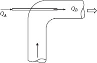
Figure P5.61 Ejector pump.
61. A jet ejector pump is shown in Figure P5.61. A high-speed stream (QA) is injected at a rate of 50 gpm through a small tube 1 in. in diameter, into a stream (QB) in a larger, 3 in. diameter, tube. The energy and momentum are transferred from the small stream to the larger stream, which increases the pressure in the pump. The fluids come in contact at the end of the small tube and become perfectly mixed a short distance downstream (the flow is turbulent). The energy dissipated in the system is significant, but the wall force between the end of the small tube and the point where mixing is complete can be neglected. If both streams are water at 60°F, and QB = 100 gpm, calculate the pressure rise in the pump.
62. Figure P5.62 illustrates two relief valves. The valve disk is designed to lift when the upstream pressure in the vessel (P1) reaches the valve set pressure. Valve A has a disk that diverts the fluid leaving the valve by 90° (i.e., to the horizontal direction), whereas the disk in valve B diverts the fluid to a direction that is 60° downward from the horizontal. The diameter of the valve nozzle is 3 in., and the clearance between the end of the nozzle and the disk is 1 in., for both valves. If the fluid is water at 200°F, P1 = 100 psig, and the discharge pressure is atmospheric, determine the force exerted on the disk for both cases A and B. The loss coefficient for the valve in both cases is 2.4 based on the velocity in the nozzle.
63. A relief valve is mounted on top of a large vessel containing hot water. The inlet diameter to the valve is 4 in., and the outlet diameter is 6 in. The valve is set to open when the pressure in the vessel reaches 100 psig, which happens when the water is at 200°F. The liquid flows through the open valve and exits to the atmosphere on the side of the valve, 90° from the entering direction. The loss coefficient for the valve has a value of 5, based on the exit velocity from the valve.
(a) Determine the net force (magnitude and direction) acting on the valve.
(b) You want to attach a cable to the valve to brace it such that the tensile force in the cable balances the net force on the valve. Show exactly where you would attach the cable at both ends.
Figure P5.62 Relief valve disk geometry.
64. A relief valve is installed on the bottom of a pressure vessel. The entrance to the valve is 4.5 in. diameter and the exit (which discharges in the horizontal direction, 90° from the entrance) is 5 in. diameter. The loss coefficient for the valve is 4.5 based on the inlet velocity. The fluid in the tank is a liquid, with a density of 0.8 g/cm3. If the valve opens when the pressure at the valve reaches 150 psig, determine
(a) The mass flow rate through the valve, in lbm/s.
(b) The net force (magnitude and direction) exerted on the valve.
(c) Determine the location (orientation) of a cable that is to be attached to the valve to balance the net force (note that a cable can support only a tensile force).
65. An emergency relief valve is installed on a reactor to relieve excess pressure in case of a runaway reaction. The lines upstream and downstream of the valve are 6 in. sch 40 pipe. The valve is designed to open when the tank pressure reaches 100 psig, and the vent exhausts to the atmosphere at 90° to the direction entering the valve. The fluid can be assumed to be incompressible, with an SG of 0.95, a viscosity of 3.5 cP, and a specific heat of 0.5 Btu/lbm°F. If the sum of the loss coefficients for the valve and the vent line is 6.5, determine
(a) The mass flow rate of the fluid through the valve in lbm/s and the value of the Reynolds number in the pipe when the valve opens.
(b) The rise in temperature of the fluid from the tank to the vent exit, if the heat transferred through the walls of the system is negligible.
(c) The force exerted on the valve supports by the fluid flowing through the system. If you could install only one support cable to balance this force, show where you would put it.
66. Consider the “tank on wheels” shown in Figure P5.66. Water is draining out of a hole in the side of the open tank, at a rate of 10 gpm. If the tank diameter is 2 ft and the diameter of the hole is 2 in., determine the magnitude and direction of the force transmitted from the water to the tank.
67. The tank in Problem 66 is 6 in. in diameter and contains water at a depth of 3 ft. On the side of the tank near the bottom is a 1.5 in. ID outlet to which is attached a ball valve, which has a loss coefficient of 1.2. When the valve is opened, the water flows out in a horizontal stream. Calculate
(a) The flow rate of the water (in gpm).
(b) The thrust exerted on the tank by the escaping water, and the direction that the tank will move. If the diameter of the outlet and valve are increased, will the thrust on the tank increase or decrease? Why?
LAMINAR FLOW
68. Use the microscopic equations of motion in Appendix E as a starting point to derive a relationship between the volumetric flow rate and the pressure gradient for a Newtonian fluid in a pipe that is valid for any orientation of the pipe axis. (Hint: the critical starting point requires that you identify which velocity and velocity gradients are nonzero, and hence the corresponding nonzero stress components, for this problem. This allows you to tailor the differential equations to suit the problem, and the resulting equations can be integrated, with appropriate boundary conditions, to get the answer.)
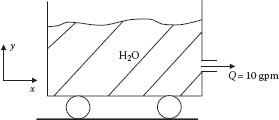
FIGURE P5.66 Water jet force on tank.
69. A viscous molten polymer is pumped through a thin slit between two flat surfaces. The slit has a depth H, width W, and length L, and is inclined upward at an angle θ to the horizontal (H≪W). The flow is laminar, and the polymer is non-Newtonian, with properties that can be represented by the power law model.
(a) Derive an equation relating the volume flow rate of the polymer (Q) to the applied pressure difference along the slit, the slit dimensions, and the fluid properties.
(b) Using the definition of the Fanning friction factor (f), solve your equation for f in terms of the remaining quantities. The corresponding solution for a Newtonian fluid can be written as f = 24/NRe. Use your solution to obtain an equivalent expression for the power law Reynolds number (i.e., NRe,pl = 24/f). Use the hydraulic diameter as the length scale in the Reynolds number.
(Note: It is easiest to take the origin of your coordinates at the center of the slit, then calculate the flow rate for one-half the slit and double this to get the answer. Why is this the easiest way?)
70. Acrylic latex paint can be described as a Bingham plastic with a yield stress of 200 dyn/cm2, a limiting viscosity of 50 cP, and a density of 0.95 g/cm3.
(a) What is the maximum thickness at which a film of this paint could be spread on a vertical wall without running?
(b) If the power law model were used to describe this paint, such that the apparent viscosity predicted by both the power law and Bingham plastic models is the same at shear rates of 1 and 100 s−1, what would the flow rate of the film be if it has the thickness predicted in (a)?
71. A vertical belt is moving upward continuously through a liquid bath at a velocity V. A film of the liquid adheres to the belt, which tends to drain downward due to gravity. The equilibrium thickness of the film is determined by the steady-state condition at which the downward drainage velocity of the surface of the film is exactly equal to the upward velocity of the belt. Derive an equation for the film thickness if the fluid is
(a) Newtonian
(b) A Bingham plastic
72. Water at 70°F flows upward through a vertical tube and overflows over the top and down the outside wall. The OD of the tube is 4 in., and the water flow rate is 1 gpm. Determine the thickness of the film. Is the flow laminar or turbulent?
73. For laminar flow of a Newtonian fluid in a tube
(a) Show that the average velocity over the cross section is half of the maximum velocity in the tube.
(b) Derive the kinetic energy correction factor for laminar flow of a Newtonian fluid in a tube (i.e., α = 2).
74. A slider bearing can be described as one plate moving with a velocity V parallel to a stationary plate, with a viscous lubricant in between the plates. The force applied to the moving plate is F, and the distance between the plates is H. If the lubricant is a grease with properties that can be described by the power law model, derive an equation relating the velocity V to the applied force F and the gap clearance H, starting with the general microscopic continuity and momentum equations. If the area of the plate is doubled, with everything else staying the same, how will the velocity V change?
75. Consider a fluid flowing in a conical section, as illustrated in Figure P5.75. The mass flow rate is the same going in (through point 1) as it is coming out (point 2), but the velocity changes because the area changes. They are related by
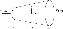
Figure P5.75 Flow in a cone.
where ρ is the fluid density (assumed to be constant here). Because the velocity changes, the transport of momentum will be different going in than going out, which results in a net force in the fluid.
(a) Derive an expression for the magnitude of this force associated with the change in momentum.
(b) Which direction will the force transmitted from the fluid to the cone act?
A |
Cross-sectional area, [L2] |
Aw |
Area of wall, [L2] |
cv |
Specific heat at constant volume, [FL/MT = L2/Mt2] |
cp |
Specific heat at constant pressure, [FL/MT = L2/Mt2] |
d |
Diameter, [L] |
D |
Diameter, [L] |
Dh |
Hydraulic diameter, [L] |
f |
Fanning friction factor, [-] |
ef |
Energy dissipated per unit mass of fluid, [FL/M = L2/t2] |
Fx |
Force component in x direction, [F = ML/t2] |
g |
Acceleration due to gravity, [L/t2] |
h |
Enthalpy per unit mass, [FL/M = L2/t2] |
Hf |
Friction (loss) head, [L] |
Hp |
Pressure head, [L] |
Hv |
Velocity head, [L] |
Hw |
Work (pump) head, [L] |
Hz |
Static head, [L] |
I |
Moment of inertia, [FLt2 = ML2] |
Kf |
Loss coefficient, [—] |
Lθ |
Angular momentum in the θ direction, [ML2/t] |
M |
Molecular weight, [M/mol] |
m |
Mass, [M] |
ṁ |
Mass flow rate, [M/t] |
P |
Pressure, [F/L2 = M/Lt2] |
Q |
Volumetric flow rate, [L3/t] |
Rate of heat transfer into the system, [FL/t = ML2/t3] |
|
q |
Heat transferred into the system per unit mass of fluid, [FL/M = L2/t2] |
R |
Gas constant, [FL/(mol T) = ML2 (mol t2T)] |
r |
Radial coordinate [L] |
s |
Entropy per unit mass, [FL/M = L2/t2] |
T |
Temperature, [T] |
t |
Time, [t] |
u |
Internal energy per unit mass, [FL/M = L2/t2] |
V |
Spatial average velocity, [L/t] |
v |
Local velocity, [L/t] |
W |
Width of plate, [L] |
Rate of work done by fluid system, [FL/t = ML2/t3] |
|
Wp |
Wetted perimeter, [L] |
w |
Work done by fluid system per unit mass of fluid, [FL/M = L2/t2] |
GREEK
α |
Kinetic energy correction factor, [—] |
β |
d/D, where d < D, [—] |
Γ |
Moment or torque, [FL = ML2/t2] |
Δ() |
()2 − ()l |
Gradient vector operator, [1/L] |
|
δ |
Film thickness, [L] |
μ |
Viscosity (constant), [M/Lt] |
v |
Specific volume, [L3/M] |
Φ |
Potential = P + ρgz, [F/L2 = M/Lt2] |
ρ |
Density, [M/L3] |
τyx |
Shear stress component, force in x direction on y area component, [F/L2 = M/Lt2] |
Shear stress tensor, [F/L2 = M/(Lt2)] |
|
τw |
Stress exerted on wall by fluid, [F/L2 = M/Lt2] |
ω |
Angular velocity, [l/t] |
SUBSCRIPTS
1 |
Reference point 1 |
2 |
Reference point 2 |
i |
Input |
o |
Output |
s |
System |
x, y, z |
Coordinate directions, [L] |
Darby, R., Viscoelastic Fluids, Marcel Dekker, New York, 1976.