10

Getting Acquainted with Lines, Rays, and Normals

Since we covered vectors in the previous chapter, it’s time to jump into exploring the mathematics of lines, rays, and normals. All three can be defined by vectors and on the surface, all appear to be the same and yet they have very specific and differing uses in graphics. Fortunately, their similarities concerning geometric structure allow them to be defined and manipulated by the same equations, as you will discover in this chapter.

The one thing lines, rays, and normals have in common is that they are all straight. This makes them very useful in graphics for defining space, direction, the edges of meshes, distance, collisions, reflections, and much more. The line construct is one of the fundamental drawing operations in graphics, as we covered in Chapter 1, Hello Graphics Window: You're On Your Way, and Chapter 2, Let’s Start Drawing.

In this chapter, we will cover the essential knowledge you need to define and manipulate lines, rays, and normals mathematically and build data structures for each into our project. We will begin with a thorough examination of the basic concepts and explore the differing uses for lines, line segments, rays, and normals. Following this, the parametric form of lines will be presented, which you will use to animate the movement of a cube from one location to another in 3D space. We will conclude this chapter by using our practical skills of drawing lines to display the normals of polygon surfaces, which is critical knowledge in understanding how surfaces are textured and lit.

To this end, in this chapter, we will cover the following topics:

• Defining lines, segments, and rays
• Using the parametric form of lines
• Calculating and displaying normals

By the end of this chapter, you will have gained a firm understanding of how these elements are used throughout graphics and be able to apply them to your projects.

Technical requirements

In this chapter, we will continue working on the project that we’ve constructed using Python, PyCharm, Pygame, and PyOpenGL.

The solution files containing this chapter’s code can be found on GitHub at https://github.com/PacktPublishing/Mathematics-for-Game-Programming-and-Computer-Graphics/tree/main/Chapter10 in the Chapter10 folder.

Defining lines, segments, and rays

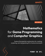
What most people call a line is a line segment. A line segment is just a piece of a line. By true mathematical definition, a line continues infinitely. In Chapter 2, Let’s Start Drawing, we used the equation for a line to draw segments between mouse clicks in our project window. Recall that the following equation was used:

y = mx + c

Here, m is the gradient (or slope) and c is the y-intercept, as shown in Figure 10.1:

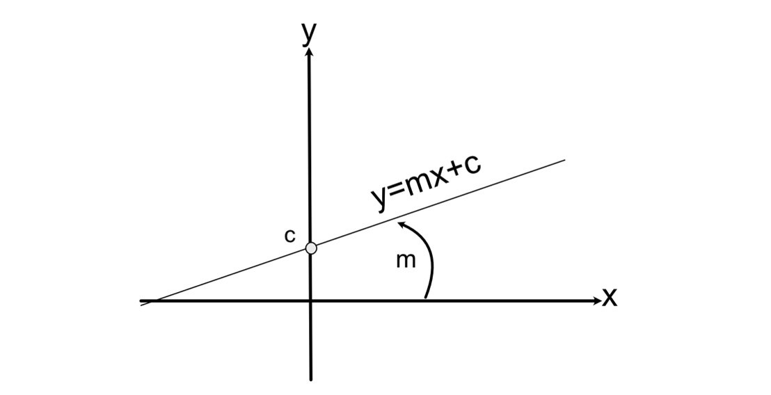
Figure 10.1: The gradient and y-intercept

The value of y can be calculated for infinite values of x and vice versa, making a line continuous. However, a line segment has a start and end, as illustrated in Figure 10.2:

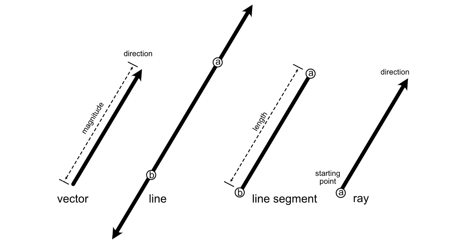
Figure 10.2: Differing straight geometrics

To clarify the difference between these straight geometrics, let’s examine their properties:

• A vector has a magnitude and direction, as we discovered in Chapter 9, Practicing Vector Essentials. It doesn’t have a location in space. Vectors are used in graphics for all manner of operations, including moving objects, measuring distances, and calculating lighting.
• A line continues to infinity from both ends. It can be defined as going through two points. A line occupies a location in space. In reality, lines aren’t used in graphics at all as it’s not possible to calculate values to infinity. However, lines can be used to calculate segments anywhere along their length for use in drawing and other calculations.
• A line segment can be defined by the same basic equation as a line but is a finite length cut off at both ends. When writing its equation, these cut-off points are featured:

This formula specifies that x is restricted to values between the x values of the cut-off points – that is, a and b. Although you might think that lines are used everywhere in graphics, line segments are more common as we don’t need to calculate straight paths to infinity. A line segment is what you see drawn on the screen and is the basic element used to draw the edges of polygons and meshes.

• A ray has a direction, like a vector, but it continues infinitely in one direction and has a definite starting point. Rays are used to specify the position and direction of lights and calculate collision detection. Rays can be defined by a starting point and using the direction of a vector.

Conceptually, you might think of lines and line segments collectively by the term line. It probably doesn’t make too much difference if that is how you understand them, so long as you grasp the concepts and can see how each is applied in graphics. I’ve already been guilty of calling them all lines, so I will continue to do so.

While lines, line segments, rays, and normals might seem fundamentally the same, you’ve now discovered how they are different. In many graphics calculations, it’s rare to use any of these elements alone, as you are about to find out.

Using the parametric form of lines

While the line equation given in the previous section is something most people are familiar with from high school mathematics, it’s not particularly useful in graphics when you want to manipulate objects or work out intersections, animations, and collisions. Therefore, we tend to use the parametric form. The parametric form of an equation, rather than using x and y to calculate positions, uses time, represented by t. This might sound confusing at first but bear with me while I explain.

Consider Figure 10.3 (a). Notice how a line segment can be represented by two points and a vector going between them:

Figure 10.3: A line segment with a vector between the start and end points

The calculation for v is as follows:

v = b – a

We can also express it like so:

b = a + v

This tells us that if we start at point a and travel along the whole length of v, we will end up at b. Where would you be if you only traveled halfway along v? This can be expressed as b = a + 0.5v. Here, you’d be at point c, as shown in Figure 10.2 (b). If you traveled no distance of v, then you’d still be at a.

The parametric form of an equation uses this scalar of v as the variable, t. So, at a, t = 0 and at b, t = 1. Therefore, the parametric equation for a line segment is as follows:

Now, just because t is restricted to values of 0 and 1 here doesn’t mean it has to be this way. If you wanted to define a line using the parametric form, you could express it like this:

This means that t can be any value at all. However, when it is 0, you’ll still have a, and when it is 1, you'll still have b. However, plugging in any other value for t will provide points along the line that extend to infinity. Therefore, t represents progress along the line from a to b, which specifies the time traveled along the vector.

Your turn…

• Exercise A:
  • What are the coordinates of the end point of a line segment where the start location is (3, 6, 7) and the vector from the start location to the end point is (1, 5, 10)?
• Exercise B:
  • What are the coordinates halfway along the line segment going from (1, 9, 5) and (10, 18, 3)?
• Exercise C:
  • What are the coordinates of a point 75% along a line segment where the end position is (2, 3, 4) and the vector from the start to the end is (5, 5, 3)?

Now, let’s use a parametric equation to linearly interpolate the position of a cube in our project to animate movement.

Let’s do it…

In this exercise, we will animate a single cube so that it moves along a line between two points using a parametric equation. This will further reinforce the use of the variable, t, to represent time:

1. Make a new folder in PyCharm called Chapter 10. Make a copy of all the files from the Chapter 9 folder and place them in this new folder. This includes Vectors.py.
2. Rename the copy of Vectors.py to Animate.py.
3. Modify the content of Animate.py, like this:

   ..

       glViewport(0, 0, screen.get_width(),

                        screen.get_height())

       glEnable(GL_DEPTH_TEST)

   trans: Transform = cube.get_component(Transform)

   start_position = pygame.Vector3(-3, 0, -5)

   end_position = pygame.Vector3(3, 0, -5)

   v = end_position - start_position

   t = 0

   trans.set_position(start_position)

   dt = 0

   trans2: Transform = cube2.get_component(Transform)

   while not done:

       events = pygame.event.get()

       for event in events:

           if event.type == pygame.QUIT:

               done = True

       if t <= 1:

           trans.set_position(start_position + t * v)

           t += 0.0001 * dt

       glPushMatrix()

       glClear(GL_COLOR_BUFFER_BIT | GL_DEPTH_BUFFER_BIT)

   ..

       glPopMatrix()

       pygame.display.flip()

       dt = clock.tick(fps)

   pygame.quit()

Here, we initially set the position of the first cube to the left-hand side of the screen, as shown in Figure 10.4, as well as after setting up the parametric equation values, including calculating v and initializing t. For this, we defined a start and end position for the movement.

There’s also a new value in there called dt. This will record the time taken for a single game loop. It gets its value from the clock.tick() function at the end of the game loop. Multiplying the movement by it (in this case, the updating value of t) will ensure the speed of movement is consistent across differing computers.

The set_position() function of the Transform class is used to set the changing position of the cube by feeding in the parametric equation.

Take note that the code for moving the cubes with the arrow keys and spacebar has been removed:

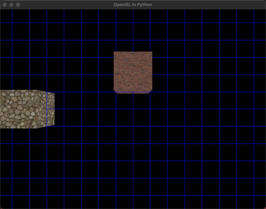
Figure 10.4: Starting position of the animated cube

4. Press play and watch the cube move across the screen, stopping when t = 1, as shown in Figure 10.5:

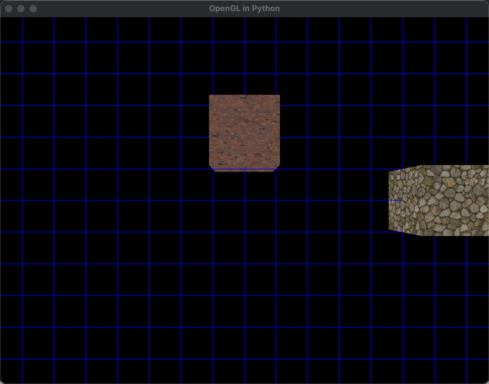
Figure 10.5: Final position of the animated cube

5. Now, modify the ending position of the line segment to (0, 0, -5), like this:

   end_position = pygame.Vector3(0, 0, -5)
6. Run the program again. The cube will stop in the center of the screen.
7. To see how values of t greater than 1 will keep the cube moving along the same line, comment out the if statement, as follows:

   #if t <= 1:
8. Run the program one more time. The cube will move across the screen and out of view on the right-hand side.

The code you’ve created in this exercise will move the cube between any two points, but make sure you put the if statement we took out previously back in.

As you’ve experienced in this section, whether we are working with points, lines, or vectors, the mathematics is the same. Sometimes, it may get confusing as to what is a vector and what is a point; the same goes for lines and line segments. Therefore, a thorough understanding of context is essential; otherwise, it just appears as though you are adding and subtracting x, y, and z values.

Other special vector-related lines (I mean this in the general sense) are normals and rays. As you will see, they too have a special place in graphics.

Calculating and displaying normals

Unlike rays, which have a starting position and direction and are infinite in length, normals are special vectors assigned to mesh surfaces and vertices. A normal is a vector that usually sits at 90 degrees to a surface. I say usually because they can be manipulated for special surface texturing effects. Normals are used to calculate how light falls on a surface, as well as define the side of a polygon to which a texture is applied. There are two places normals are used; on surfaces and vertices, as shown in Figure 10.6, though usually, they are defined with vertices in mesh files:

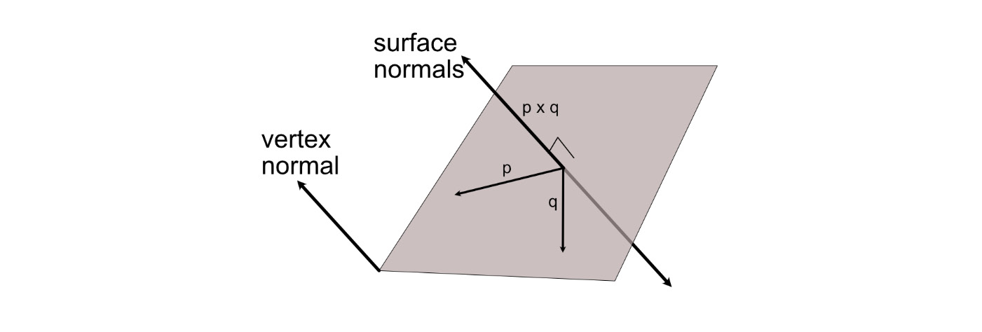
Figure 10.6: Normals

As shown in Figure 10.6, mathematically, a plane has two normals, which can be found using the cross product of two vectors on the surface. Recall from Chapter 9, Practicing Vector Essentials, that multiplying two vectors together results in a third vector that sits at right angles to the initial vectors. In Figure 10.6, one of the surface normals can be found with q x p and the other with p x q. In graphics, there’s usually only a normal on one side of a plane. This helps define the front side of a polygon. Figure 10.7 shows a mesh in Maya displaying the surface and vertex normals:

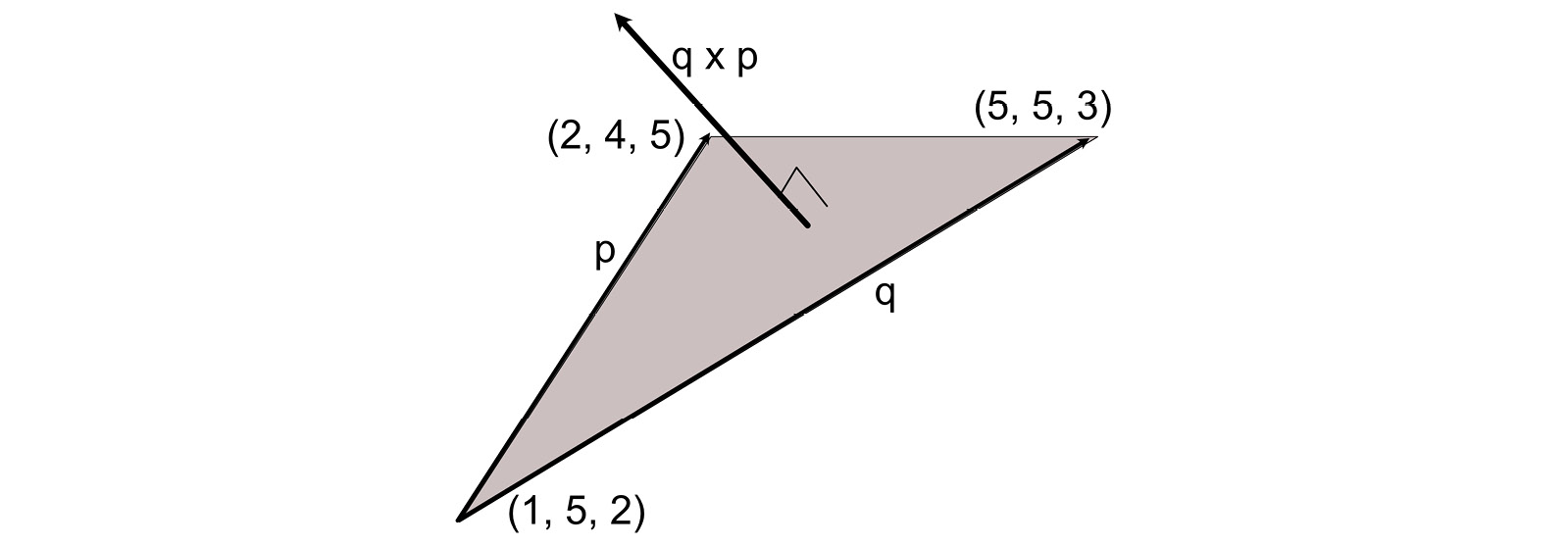
Figure 10.7: Face and vertex normals on a mesh

To calculate a normal, given a triangle that represents one of the flat surfaces in a mesh, two vectors that run between the vertices can be calculated to find vertexes that sit flush with the surface. Then, they can be crossed together to get the normal.

For example, given the triangle in Figure 10.8, the vectors of p and q can be calculated using the vertex values:

Figure 10.8: Calculating the normal of a triangle

Here, we have the following:

p = (2, 4, 5) – (1, 5, 2) = (1, -1, 3)

q = (5, 5, 3) – (1, 5, 2) = (4, 0, 1)

q x p = (q.y * p.z – q.z * p.y), (q.z * p.x – q.x * p.z), (q.x * p.y – q.y * p.x)

q x p = (1, -11, -4)

Note that the normal is a vector, so it does not need to originate anywhere special on the surface. It only has a direction and magnitude.

Your turn…

• Exercise D:
  • What are the normal vectors for the vectors v = (8, 2, 3) and w = (1, 2, 3)? What observation can you make about the values contained in the two normals?
• Exercise E:
  • What are the normal vectors for the triangle defined by the vertices a = (3, 1, 2), b = (9, 5, 2) and c = (15, 8, 7)?

Let’s try calculating and displaying some normals for the cubes we’ve been working with throughout this project.

Let’s do it…

In this exercise, we will take some of the vertices of the cubes we’ve been working on and calculate the normals to display. Follow these steps:

1. Create a new Python script called MathOGL.py. We will use this file to code some mathematical functions.
2. Let’s start by adding functions to MathOGL.py with a cross-product calculation, like this:

   import pygame

   def cross_product(v, w):

       return pygame.Vector3((v.y*w.z - v.z*w.y), 

                             (v.x*w.z - v.z*w.x), 

                             (v.x*w.y - v.y*w.x))

You’ll recognize the cross-product equation we examined in Chapter 9, Practicing Vector Essentials.

3. Create a new Python script called DisplayNormals.py. This file will house a new class that can be added to an object to display the normals.
4. Add the following code to DisplayNormals.py:

   import pygame

   from OpenGL.GL import *

   from MathOGL import *

   class DisplayNormals:

       def __init__(self, vertices, triangles):

           self.vertices = vertices

           self.triangles = triangles

           self.normals = []

           for t in range(0, len(self.triangles), 3):

               vertex1 = self.vertices[self.triangles[t]]

               vertex2 = self.vertices[self.triangles[t +

                                                      1]]

               vertex3 = self.vertices[self.triangles[t + 

                                                      2]]

               p = pygame.Vector3(

                   vertex1[0] - vertex2[0],

                   vertex1[1] - vertex2[1],

                   vertex1[2] - vertex2[2])

               q = pygame.Vector3(

                   vertex2[0] - vertex3[0],

                   vertex2[1] - vertex3[1],

                   vertex2[2] - vertex3[2])

               norm = cross_product(p, q)

               nstart = (0, 0, 0)

               self.normals.append((nstart, nstart + 

                                    norm))

The initialization method of DisplayNormals.py accepts the vertices and triangles that will be passed when the class is instantiated later. We use the vertices of the triangle to create two vectors that define two sides of the triangle. These vectors, p and q, are then run through the cross-product method to return a normal vector.

The normals that have been calculated are stored in an array as a line segment. In this case, we are drawing the normal from (0, 0, 0), which is the center of the cube, out to the length of the normal:

    def draw(self):
        glColor3fv((0, 1, 0))
        glBegin(GL_LINES)
        for i in range(0, len(self.normals)):
            start_point = self.normals[i][0]
            end_point = self.normals[i][1]
            glVertex3fv((start_point[0],
                         start_point[1], 
                         start_point[2]))
            glVertex3fv((end_point[0], end_point[1], 
                         end_point[2]))
        glEnd()

The draw method sets the drawing color to green and then, using the GL_LINES setting, draws the normal as a line segment. Here, start_point and end_point are defined as separate variables to make the code more readable.

5. In Object.py, make the following modifications:

   ..

   from Grid import *

   from DisplayNormals import *

   class Object:

       def __init__(self, obj_name):

   ..

   elif isinstance(c, Grid):

               c.draw()

        elif isinstance(c, DisplayNormals):

              c.draw()

        elif isinstance(c, Button):

   ..

Here, we are adding the ability for the Object update method to handle DisplayNormal type components.

6. Finally, we have to update the main program in Animate.py to add the normals to a cube. Open this file and make the following modifications:

   ..

   from Cube import *

   from Grid import *

   from DisplayNormals import *

   from pygame.locals import *

   ..

   cube = Object("Cube")

   cube.add_component(Transform((0, 0, -5)))

   cube.add_component(Cube(GL_POLYGON, "images/wall.tif"))

   cube.add_component(DisplayNormals(

                      cube.get_component(Cube).vertices, 

                      cube.get_component(Cube).triangles))

   cube2 = Object("Cube")

   cube2.add_component(Transform((0, 1, -5)))

   ..

This new code will ensure that a DisplayNormals component is added to the cube. Note that the Cube component, which holds the vertices and triangles, is required to pass the vertices and triangles through to the DisplayNormals instance.

7. Running this code will show the animated cube displaying each of its green normals, as shown in Figure 10.9:

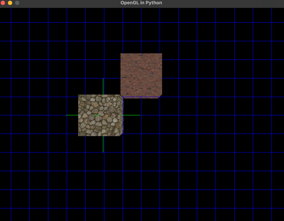
Figure 10.9: A cube displaying its normals

Your turn…

• Exercise F:
  • In the previous exercise, we added a class to display the normals on a cube in the project. This code only draws one of the normals. Modify the code so that it calculates and draws both normals.

In this section, we’ve only touched on the concept of normals by learning to calculate and draw them. Understanding how to do this will help you as you move forward with your learning journey in graphics.

Summary

By now, I am sure you are gaining an appreciation of the importance of vectors, and just how important it is for graphics and game developers to have a firm grasp of them both conceptually and practically. Trust me, this chapter won’t be the last time you see them. The mathematical concepts we explored in this chapter might appear to cover the same ground over and over concerning calculating points and vectors, but this should only convince you further how important these methods are.

Lines are far more complex than they first seem. Although most straight geometrical elements are called lines in a general, collective sense, the differences between vectors, lines, line segments, and rays are clear. Each has its place in graphics development in data structures and drawing, though we can apply many of the same mathematical calculations to any of them. Is it any wonder that many of these are stored in the same data structure of pygame.Vector3?

We started this chapter by defining the concepts of lines, line segments, rays, and normals. Next, we took this knowledge and applied it to constructing parametric line equations, which were then used in our project to animate a cube so that it moves across the screen. Following this, line drawing was applied to the display of normals to help you visualize the front and back sides of a polygon.

In the next chapter, we will continue using lines, vectors, and rays to further explore the function of normals in drawing, texturing, and lighting 3D objects.

Answers

Exercise A:

end = start + v

end = (3, 6, 7) + (1, 5, 10)

end = (4, 11, 17)

Exercise B:

v = (10, 18, 3) – (1, 9, 5)

v = (9, 9, -2)

t = 0.5

point = (1, 9, 5) + 0.5 * (9, 9, -2)

point = (1, 9, 5) + (4.5, 4.5, -1)

point = (5.5, 13.5, 4)

Exercise C:

start position = (2, 3, 4) – (5, 5, 3) = (-3, -2, 1)

t = 0.75

point = (-3, -2, 1) + 0.75 * (5, 5, 3)

point = (-3, -2, 1) + (3.75, 3.75, 2.25)

point = (0.75, 1.75, 3.25)

Exercise D:

(8, 2, 3) x (1, 2, 3) = (2*3 – 3*2, 3*1 – 8*3, 8*2-2*1)

= (0, -21, 14)

(1, 2, 3) x (8, 2, 3) = (2*3 – 3*2, 3*8 – 1*3, 1*2- 2*8)

= (0, 21, -14)

These two vectors are direct opposites. They are parallel but pointing in opposite directions, which is what you expect from the two normals. You can tell this by looking at the x, y, and z values, each of which has the same values but is signed differently.

Exercise E:

To begin solving this, you need two vectors. These can be calculated from the vertices, as shown in Figure 10.10.

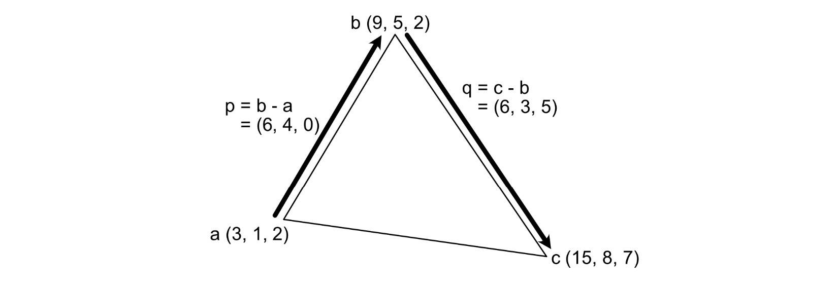
Figure 10.10: Calculating the vectors on a triangle

Then, the cross products are found of p x q and q x p, like this:

p x q = (4*5-0*3, 0*6-6*5,6*3-4*6) = (20, -30, -6)

q x p = (3*0-5*4, 5*6-6*0, 6*4-3*6) = (-20, 30, 6)

Notice once again that each normal has the same values, just with different signs.

Exercise F:

To calculate and draw both normals for each of the triangles in the cube, we must add another cross-product calculation and add the extra vector to the normals array, like this:

norm1 = cross_product(p, q)

norm2 = cross_product(q, p)

nstart = (0, 0, 0)

self.normals.append((nstart, nstart + norm1))

self.normals.append((nstart, nstart + norm2))