13
Understanding the Importance of Matrices
Matrices are an advanced mathematical concept that you will find everywhere throughout computer games and graphics. Their power comes from their ability to store affine transformations and apply them through multiplication. An understanding of their inherent structure and mathematical operations will provide you with a deep appreciation of the methods underpinning all graphics and game engines.
In this chapter, we will cover the following topics:
- Defining matrices
- Performing Operations on matrices
- Creating matrix representations of affine transformations
- Combining transformation matrices for complex maneuvers
We will begin by defining matrices and working through all the mathematical operations that can be performed on them. Then, we will examine how the affine transformations presented in Chapter 12, Mastering Affine Transformations, can be achieved through matrix operations. This will involve clarifying the benefits and use of working with matrices in a format called homogeneous representation. Finally, you will practice manually calculating transformations with matrices while using your OpenGL Python project to reveal the matrices it uses to manipulate the objects you’ve been drawing.
By the end of this chapter, you will have discovered how valuable matrices are in computer graphics and be comfortable using them to define compound affine transformations.
Technical requirements
In this chapter, we will be using Python, PyCharm, and Pygame, as used in previous chapters.
Before you begin coding, create a new folder in the PyCharm project for the contents of this chapter called Chapter_13.
The solution files for this chapter can be found on GitHub at https://github.com/PacktPublishing/Mathematics-for-Game-Programming-and-Computer-Graphics/tree/main/Chapter13.
Defining matrices
A matrix is an array of numbers. It is defined by the number of rows and columns that define its size. For example, this is a matrix with three rows and two columns:

Each value in the matrix is associated with its location. The value of 3 in the preceding matrix is located in row 0, column 0. More formally, we write the following:

![]()
The values specified in the square brackets are in the order [row, column], like so:
![]()
![]()
Here, the value in row 2, column 1 is 1, and the value in row 1, column 0 is 4.
In pure theoretical mathematics, the row and column values start at 1. We are starting our count at 0 because, in programming, when storing arrays and matrices, the index values start at 0.
Now, let’s take a look at the mathematical operations that can be achieved with two matrices.
Performing operations on matrices
All matrix manipulation occurs via a set of mathematical operations based on addition, subtraction, and multiplication. Because matrix operations use these familiar fundamentals of arithmetic, they are a relatively easy concept to grasp. In this section, you will explore each of these, beginning with addition, subtraction, and multiplication. However, when it comes to division, as you will soon experience, a whole new set of concepts are required. We will cover these toward the end of this section.
Go easy on yourself if you haven’t worked with matrices before and become overwhelmed with the content. They take a lot of practice to become comfortable with and you may not appreciate many of them until you get to apply them in your own graphics projects.
Let’s start with the very familiar and simple addition and subtraction operations.
Adding and subtracting matrices
To add or subtract two matrices, they must be the same size. Matrices are considered the same size when they have the same number of rows and columns. To add the values, the numbers in the same locations are added together and placed in a resulting matrix of the same size; for example:

Here, you can see how the value 3 in the first matrix at position [0, 0] is added to the value 1 in [0, 0] in the second matrix, and that the result of 3 + 1 is placed into the solution at [0, 0]. The same operation occurs for all values in both matrices until the solution matrix is complete.
Subtracting matrices occurs in the same way, except that the values in the second matrix are subtracted from those in the first matrix; for example:

As well as being able to add and subtract matrices, they can be multiplied by a value.
Multiplying by a single value
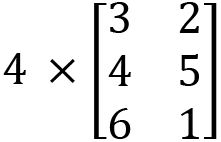
A matrix can be multiplied by a single number called a scalar. This scalar value is multiplied by all the values in the matrix. The size of the resulting matrix is the same as the original one; for example:
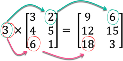
Notice that the result goes into the same position in the resulting matrix as the multiplied value from the original. Here, you can see that the value of 2 at position [0, 1], when multiplied by 3 (the scalar), goes into the position where 6 is in the result at [0, 1].
Multiplying by a single value is straightforward. Something a little more complex is multiplying one matrix with another.
Multiplying one matrix with another
Two matrices can only be multiplied together when the first matrix’s number of columns is the same as the second matrix’s number of rows. In the case of the following example, the first matrix has three columns, and the second matrix has three rows:

The resulting matrix will have the same number of rows as the first matrix and the same number of columns as the second matrix. In this case, multiplying the first matrix, which has a size of 2 x 3, with the second matrix, which has a size of 3 x 2, will produce the resulting matrix, which is 2 x 2.
Also, note that in the equation, the two matrices do not require a multiplication sign between them. Instead, a single dot is used – not a full stop, but a vertically centered dot. The reason for this is that the operation of multiplying matrices like this is called the dot product. This is the very same operation we used to calculate the angle between vectors in Chapter 9, Practicing Vector Essentials. But what does this look like for matrix multiplication? Let’s take a look. First, we will strip the matrices of values and use position holders instead, like this:

The calculations take place by working out the dot product between each row in the first matrix with each column in the second matrix, like so:
![]()
![]()
![]()
![]()
In the next section, we will be moving on to something far more complicated to do with matrix operations, so it’s probably a good time to pause and reflect on what you’ve learned so far with a few exercises.
Your turn…
Exercise A. Calculate the following:

Exercise B. Calculate the following:

Exercise C. Calculate the following:
Exercise D. Calculate the following:

Exercise E. Calculate the following:

Dividing matrices
You cannot divide one matrix by another. Truly! There’s no equation for performing a division between matrices. Instead, we must perform a multiplication, like this:
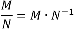
But what is ![]() ? It means the inverse of the matrix N. If a matrix is multiplied by its inverse, then the resulting matrix is an identity matrix, like so:
? It means the inverse of the matrix N. If a matrix is multiplied by its inverse, then the resulting matrix is an identity matrix, like so:
![]()
I bet you have more questions right now. And rightly so. This section is a trip down the rabbit hole in which you are going to learn a lot of new terminology and concepts before we answer the initial question of solving matrix division.
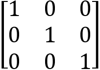
An identity matrix is a square matrix with 1s on the diagonal and 0s everywhere else. A square matrix is one where the number of rows equals the number of columns. Therefore, a matrix of size 3 x 3 is considered square. An identity matrix of this size would look like this:
If you’re thinking you’ve heard the word identity before in this book, that’s because you have – specifically, in Chapter 7, Interactions with the Keyboard and Mouse for Dynamic Graphics Programs. Remember this line of code?
glLoadIdentity()In OpenGL, it does exactly what its name suggests – it loads an identity matrix onto the matrix stack. This is another term that may be new to you, but we won’t go into that right now as it will complicate things; we’ll leave this until Chapter 14, Working with Coordinate Spaces.
The fact that a matrix multiplied by its inverse results in an identity matrix is an interesting fact but it doesn’t help us calculate the inverse matrix. Instead, to find the inverse matrix, we have to calculate the matrix’s determinant.
Calculating the determinant
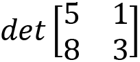
The determinant is a special value that can be calculated from a square matrix. It is useful in working with linear equations, calculus, and, more importantly for us, finding the inverse of a matrix. For a 2 x 2 matrix, the determinant can be found by multiplying the opposite values, and then taking one result away from the other, like this:

The following is an example:

If you consider the operation we’ve just performed visually, we are multiplying values in a criss-cross manner, like this:
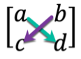
Now, there is a sane reason for looking at the operation like this: it will help us work out the determinant for larger matrices as their calculations become more complex. Let’s take a look at a 3 x 3 matrix:

If the calculation looks rather nasty, then consider it visually, as we did with the 2 x 2 matrix:

You might read this as the determinant using each of the values in the top rows as scalars for the determinants of the 2 x 2 matrix composed of the values in the other rows, which aren’t in the same column as the scalar value.
For determinants of larger matrices, check out https://mathinsight.org/determinant_matrix. For a quick determinant calculation, try https://matrix.reshish.com/determinant.php.
Your turn…
Exercise F. Calculate the following:
Exercise G. Calculate the following:

Calculating the inverse
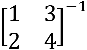
Now that we can calculate the determinant, how do we use it to find the inverse of a matrix? The formula is as follows:

Putting this into words, the inverse of a matrix is 1 over the determinant multiplied by a matrix constructed from the original, which has the a and d values swapped and the b and c values negated.
Let’s try working with this example:

How do we know whether this is correct? Well, remember that a matrix multiplied by its inverse will result in the identity matrix. Therefore, we can perform the following calculation to check:

The result will always give you an identity matrix.
Your turn…
Exercise H. Calculate the following:
Calculating the division
At the beginning of this section, we set out to calculate the division of two matrices, which we later found out wasn’t possible. Instead, we need to perform multiplication, like so:

Now that we know how to find the inverse of a matrix, we can perform division; for example:


Instead of explicitly performing a division, the result is obtained by multiplying one matrix with the inverse of the divisor matrix.
Your turn…
Exercise I. Calculate the following:

This section has presented a brief overview of the mathematical operations that can be performed with matrices, as well as revealing the new concepts of determinants and identity matrices. While only about half of this chapter is devoted to examining these concepts, this should give you a powerful skill set that will greatly enhance your ability to work with graphical applications, from animations and shader coding to artificial intelligence. This content is usually delivered to students in several university-level subjects, but unfortunately, there’s only limited space in a book that covers mathematics across the breadth of computer graphics to examine them in detail. Having said that, I strongly encourage you to explore the topic further. To this end, I have provided some extra learning resources.
Extra learning resources
Use the following links to practice and strengthen your understanding of matrix mathematics:
https://www.mathsisfun.com/algebra/matrix-introduction.html
https://www.khanacademy.org/math/algebra-home/alg-matrices
https://www.cs.mcgill.ca/~rwest/wikispeedia/wpcd/wp/m/Matrix_%2528mathematics%2529.htm
Thus far, we’ve examined matrices from a theoretical viewpoint, and you’ve been able to explore the operations that are used to manipulate them and calculate values. But what do any of the values mean? Without context, they are just fancy data structures.
The true power of matrices cannot be fully appreciated until they are used in a practical setting. They are used throughout computer graphics because of the way they store information, as well as the power that can be achieved when they’re multiplied. There’s no better place to see this applied than when they are used to represent affine transformations.
Creating matrix representations of affine transformations
In Chapter 12, Mastering Affine Transformations, we examined numerous techniques for repositioning and resizing vertices and meshes. The mathematics involved, except for rotations, was mostly straightforward. For these formulae, we applied straightforward arithmetic and some trigonometry to build up equations. Would it surprise you to know that you can represent these transformations as matrix operations? In this section, I will reveal how this can be achieved.
Moving from linear equations to matrix operations
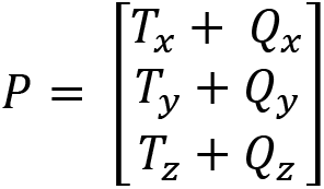
Let’s remind ourselves of the formulae used for the most popular of the affine transformations – translation, scaling, and rotation. The point, Q, can be translated by adding a translation value, T, to each of its coordinates, resulting in a new point, P:
P(x, y, z) = T(x, y, z) + Q(x, y, z)
We can turn this into a matrix addition operation like so:

If you are thinking that I’ve only turned these into arrays and not matrices, then you’d be incorrect. An array is a one-dimensional matrix. It either has one row or one column, depending on its orientation. If you remember back to earlier in this chapter, in the Adding and subtracting matrices section, when we looked at additions with matrices, you learned how the values add together to result in the P matrix. In the same way, we performed a translation with linear equations:
We can also turn a scaling transformation into a matrix operation. Recall that the scaling formula is as follows:
P(x, y, z) = S x Q(x, y, z)
It can also be written like so:
P(x, y, z) = S(x, y, z) x Q(x, y, z)
This demonstrates that the scale that’s applied to x, y, and z of the Q point can be all the same value or different values. This can be turned into a matrix multiplication operation like so:
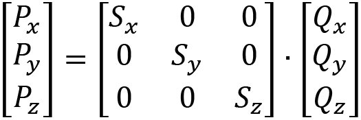
Let’s expand this using the matrix multiplication method so that you can see the result is to multiply the correct values together to gain a scaling operation:
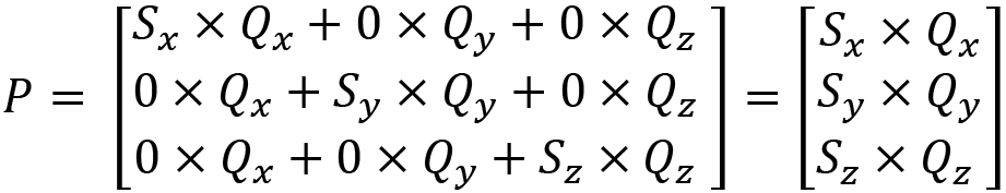
So, it’s a little more complex than addition, but it does perform scaling with matrices.
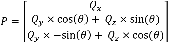
Finally, we have rotation. This is inherently more difficult because rotation has three different operations, depending on the axis of rotation. Recall the rotation operations for an X-axis roll:
![]()


Just like for scaling, we want to consider the operations that are being performed on each of the x, y, and z coordinates so that we can place the operations in the correct location in a matrix. These operations, when converted into matrix multiplication, turn three separate formulas into one:
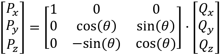
Can you see how the three separate equations for an x pitch are contained within this matrix multiplication? If you do the multiplication, you will end up with this:
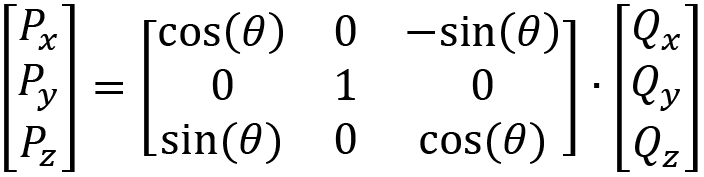
The separate formulas for the Y-axis are as follows:
![]()

![]()
When the Y-axis rotation formulas are condensed into a matrix multiplication, we get the following:
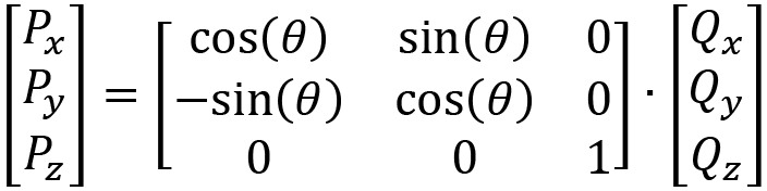
Finally, we can take the equations for a Z-axis roll:


![]()
When the Z-axis rotation formulae are merged into a matrix multiplication, we get the following:
Wow – a lot of mathematics has just been presented in this section. Take your time understanding it as it’s an exceptionally important concept in computer graphics. It might seem like a lot of fuss over nothing and a way to complicate all the calculations, but it endeavours to make them easier, as you will see in the next section.
Compounding affine transformations
Thus far, we have converted the affine transformation equations that were revealed in Chapter 12, Mastering Affine Transformations, into matrix operations. Take another look at them. What is similar or not similar in the results for the individual transformations? The difference I’d like you to spot is that the translate matrix operations involve adding one-dimensional matrices, whereas the scaling and rotation operations are multiplications with 3 x 3 matrices.
If you didn’t know, the fastest mathematical operation a computer can perform is multiplication. So, if we want to start mixing translation, scaling, and rotation, it would make sense for the three to be in the same format so that we can achieve smooth multiplication between them. In OpenGL, when a series of glTranslate(), glScale(), and glRotate() commands are executed, they are multiplied together into the same matrix. So, how does this happen?
Enter homogeneous representation. By adding a fourth component to the end of points and vectors to create what’s called a homogenous coordinate, all three transformation matrices can be multiplied. This works by adding a value of 0 to the end of a vector’s representation and a 1 to a point. For example, the vector (8, 3, 4) becomes (8, 3, 4, 0) and the point (1, 4, 3) becomes (1, 4, 3, 1). The last component is given a designation of w so that a vector or point is represented by (x, y, z, w).
How does this change the transformation matrices? Well, the translation becomes as follows:

Expanding this, you can see how the addition operation of translation is maintained:
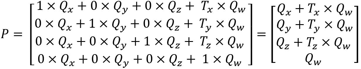
If a point is being translated, the value of ![]() will be 1 and the beforehand matrix can be simplified like so:
will be 1 and the beforehand matrix can be simplified like so:
If a vector is being translated, the value of ![]() will be 0 and the beforehand matrix can be simplified like so:
will be 0 and the beforehand matrix can be simplified like so:

As you can see, a point will be moved, whereas a vector will retain its original value. This works with point and vector mathematics as points can be moved, but vectors can’t as they don’t represent a location in space. If you were to move a vector, it would retain its original value as it simply represents direction and magnitude, not location.
Now that the translation operations have been converted into a homogeneous representation, it can be multiplied by the scaling and rotation matrices in any required order. However, before this can happen, both the scaling and rotation matrices also need to become homogenous. For scaling, the operation becomes as follows:

The following is for an X-pitch rotation:

For a Y-yaw rotation:

For a Z-roll rotation:

Now that you know how to represent the transformation functions in homogeneous coordinates, it’s time to examine how they can be multiplied together.
Combining transformation matrices for complex maneuvers
As with the OpenGL order of transformations, which we discussed in Chapter 12, Mastering Affine Transformations, when combining these homogeneous representation matrices to produce compound movements involving translation, scaling, and rotation, the matrices are presented in reverse order. For example, to transform a point by (3, 4, 5), rotate it around the X-axis by 45 degrees, and then scale it by 0.3 in all directions; the matrix multiplication is as follows:
Note how the translation matrix of the first operation is placed on the right and the scaling matrix on the left. To multiply this out, we begin by multiplying the last two matrices (the translation and rotation) to get the following:

Then, we complete the multiplication with the remaining two matrices, which results in the following:

Although learning to calculate these operations by hand is a great skill to have and will help embed your understanding of them, I’m not going to ask you to do it here. You will, however, now get a chance to examine these operations in OpenGL and use an online calculator to validate the results.
Let’s do it…
In this practical exercise, you will create a transformation in your OpenGL Python project and compare the values obtained in the matrices in the program with those calculated manually:
- Create a new Python folder called Chapter_13 and copy the contents from Chapter_12 into it.
- Make a copy of ExploreNormals.py and call it TransformationMatrices.py.
- Modify the code in TransformationMatrices.py to draw just a single textured cube positioned at the origin:
import math
from Object import *
from pygame.locals import *
from OpenGL.GLU import *
from Cube import *
In the first part of the code, notice the reduction in the number of required libraries.
In the second part of the code, ensure you have only one cube being drawn, as follows:
..
done = False
white = pygame.Color(255, 255, 255)
objects_3d = []
objects_2d = []
cube = Object(“Cube”)
cube.add_component(Transform((0, 0, 0)))
cube.add_component(Cube(GL_POLYGON,
                   “images/wall.tif”))
objects_3d.append(cube)
clock = pygame.time.Clock()
fps = 30
..
Ensure you position it at (0,0,0), and use whatever image you’ve been putting on the cubes thus far, instead of the wall.tif one that I am using.
The rest of the program remains the same.
When the code is run, the window will be filled with the texture of the cube when the camera is near it, as shown in Figure 13.1:
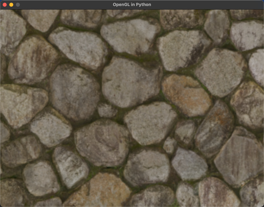
Figure 13.1: Render of a cube at the origin
- In Object.py, re-instantiate the scaling, rotation, and translation lines if you commented them out previously:
def update(self, events = None):
glPushMatrix()for c in self.components:if isinstance(c, Transform):pos = c.get_position()scale = c.get_scale()rot_angle = c.get_rotation_angle()rot_axis = c.get_rotation_axis()glTranslatef(pos.x, pos.y, pos.z)glRotated(rot_angle, rot_axis.x,rot_axis.y, rot_axis.z)glScalef(scale.x, scale.y, scale.z)elif isinstance(c, Mesh3D):glColor(1, 1, 1) - Back in TransformationMatrix.py, add the following transformations to the cube:
..
cube = Object(“Cube”)
cube.add_component(Transform((0, 0, 0)))
cube.add_component(Cube(GL_POLYGON,
“images/wall.tif”))trans: Transform = cube.get_component(Transform)
trans.set_position((0, 0, -3))
trans.set_rotation_axis(pygame.Vector3(1, 0, 0))
trans.update_rotation_angle(45)
trans.set_scale(pygame.Vector3(0.5, 2, 1))
objects_3d.append(cube)
clock = pygame.time.Clock()
..
When you run the code now, the cube will have moved slightly back into the screen, rotated by 45 degrees around the X-axis, halved in the x direction, and doubled the size in the y direction, as shown in Figure 13.2:
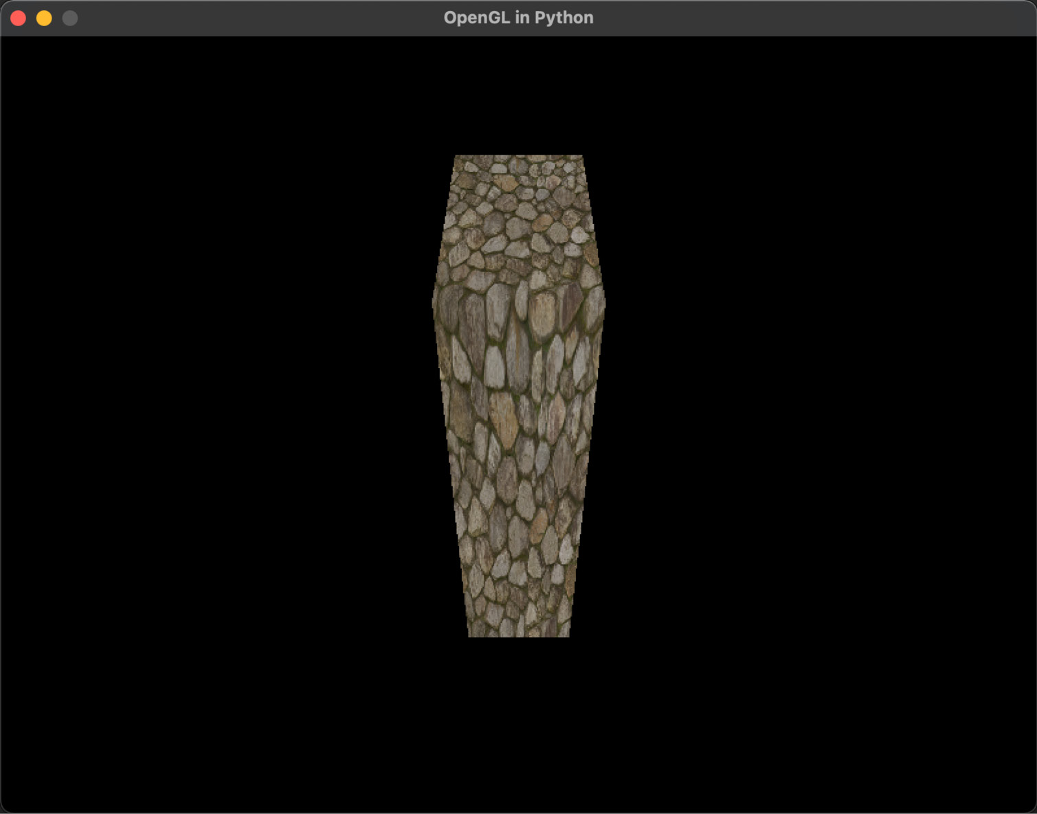
Figure 13.2: The cube after adding transformations
- Take a look at Object.py and look at the order of execution of the translation, rotation, and scaling:
glTranslatef(pos.x, pos.y, pos.z)glRotated(rot_angle, rot_axis.x,rot_axis.y, rot_axis.z)glScalef(scale.x, scale.y, scale.z)
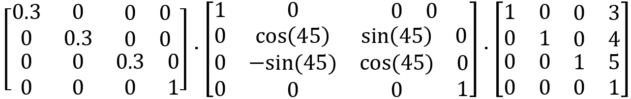
Given that these will execute in reverse order, the matrix multiplication with the values you fed into these operations in step 5 will be as follows:

- You can calculate the result of the multiplication given in step 6 manually or use the handy online Matrix Multiplication Calculator tool available at https://matrix.reshish.com/multCalculation.php.
Because there are three matrices to multiply, we begin with the two on the right. Although I’ve said matrix multiplication happens backward, here, we start with the two right-most matrices and multiply these going from left to right, as shown in Figure 13.3:
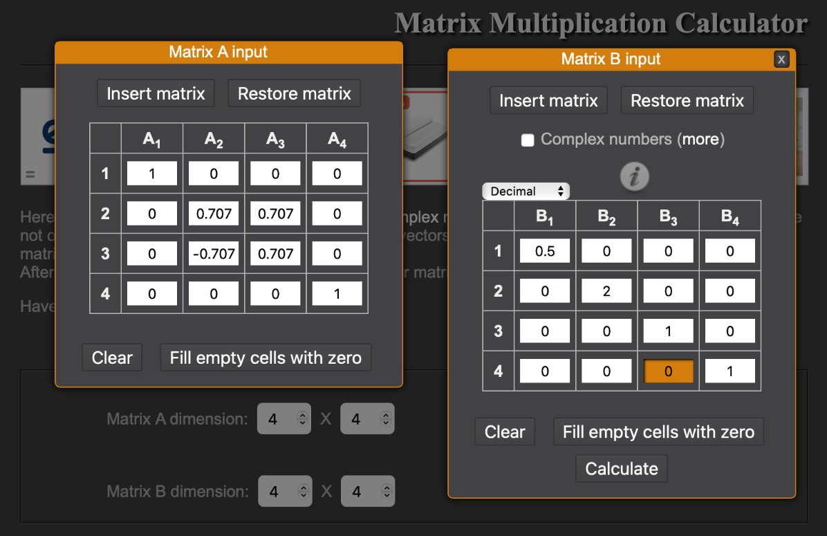
Figure 13.3: Calculating rotation with translation
For this first calculation, note that both matrices are 4 x 4 in size and the cosine and sine, which are at 45 degrees, have already been determined as 0.707. Once this operation is complete, the resulting matrix can be multiplied with the scaling matrix, as shown in Figure 13.4. Ensure that you put the scaling matrix to the left:
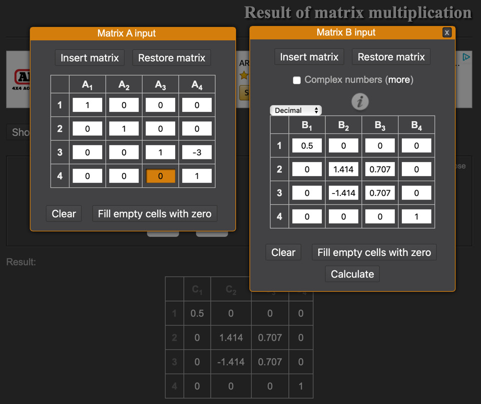
Figure 13.4: Calculating scale with the pre-calculated rotation/translation matrix
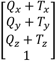
On calculating this, the matrix shown in Figure 13.5 will be displayed:
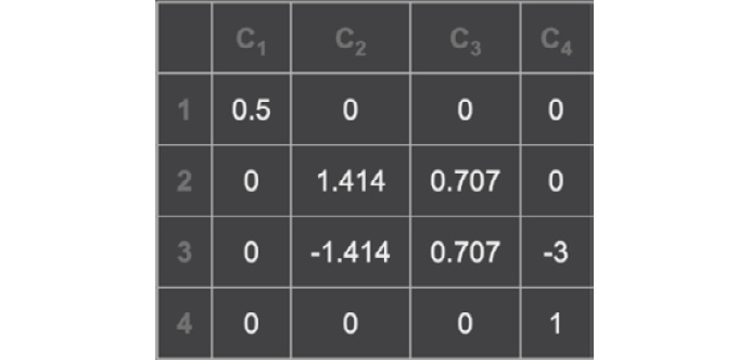
Figure 13.5: The result of multiplying the translation, rotation, and scaling matrices
- To validate this calculation, we can also ask OpenGL what it has stored in our program. The internal OpenGL matrix that holds all the transformation multiplications is called the ModelView Matrix. We can obtain its value by adding the following code to Object.py after the transformations have been applied:
rot_axis = c.get_rotation_axis()glTranslatef(pos.x, pos.y, pos.z)glRotated(rot_angle, rot_axis.x, rot_axis.y,rot_axis.z)glScalef(scale.x, scale.y, scale.z)mv = glGetDoublev(GL_MODELVIEW_MATRIX)print(“MV: “)print(mv)elif isinstance(c, Mesh3D):
After adding this code, run the program. The ModelView Matrix will display on a loop in the console. Once you see it, you can stop running the program. In the console, you should see the following output:
MV:
[[ 0.5         0.          0.          0.        ]
 [ 0.          1.41421354  1.41421354  0.        ]
 [ 0.         -0.70710677  0.70710677  0.        ]
 [ 0.          0.         -3.          1.        ]]
The matrix will be transposed (the rows and columns will be switched) as that’s how OpenGL works with them, but you’ll see the results are identical to those we calculated by hand.
As you’ve seen in this section, matrices are a powerful concept for storing transformational information for 3D objects. While they are laborious to calculate manually, it can be a valuable exercise to sometimes question the outputs from a program against hand-performed calculations and vice versa, to assist you in catching any potential errors. That was the purpose of the practical exercise you’ve just completed.
Summary
A lot of mathematical concepts were covered in this chapter that focused on matrices. Besides understanding vectors, a solid knowledge of matrices (especially 4 x 4) is an essential skill to have as a graphics programmer since they underpin the majority of the mathematics found in graphics and game engines. Once you appreciate the beauty of their simplicity and power, you’ll become more and more comfortable with their use.
In this chapter, we have only scratched the surface of using matrices in graphics. After learning how the addition operation that’s used in translations can be transformed into a 4 x 4 matrix, and integrated with scaling and rotation to perform compound transformations in 3D, we took a brief look at the ModelView Matrix in OpenGL using the project code created thus far. However, the way we currently perform the transformations is restricted to the same order as how glTranslate(), glRotate(), and glScale() are used in the existing code.
In the next chapter, we will dig deeper into the matrices used in OpenGL for manipulating objects – not only with the transformations we’ve been working with thus far but also the camera position and orientation, the projection modes, and allowing more complex compound transformations not restricted by a set coding order. These are the next essential steps in your learning journey, as you’ll be moving toward understanding the coordinate spaces used in graphics for displaying 3D objects. This will give you an appreciation of advanced vertex shaders.
Answers
For a great online matrix calculator that will also reveal the working out for you, visit https://matrix.reshish.com/multiplication.php:
Exercise A:

Exercise B:
Exercise C:

Exercise D:
Exercise E:

Exercise F:

Exercise G:

Exercise H:

Exercise I:


