
Chapter 24. Root Locus Techniques
As we saw in Chapter 23, the location of the poles and zeros of the transfer function determines the system’s dynamic behavior. We can therefore change the dynamics of the system by moving the poles and zeros to more desirable positions, a method known as “pole placement.” The easiest way to do this is by adjusting the controller gains—that is by “tuning” the controller. (See Chapter 9 for more hands-on techniques of controller tuning.)
As the controller gains are varied, the poles and zeros of the closed-loop transfer function trace out curves in the complex plane that are called root locus curves. A root locus diagram is a plot of the complex plane showing the root locus curves[25] as the gain is increased from zero toward infinity. Given such a diagram, we can choose the gain value that moves the dominant poles closest to their desired locations.
Because the structure of transfer functions is not arbitrary (they tend to be rational polynomials), we can make some general statements about global features of the corresponding root locus diagrams. These rules are discussed next.
Construction of Root Locus Diagrams
Root locus diagrams are usually drawn for closed-loop systems, such as the one depicted in Figure 24-1. This system has the closed-loop transfer function

This function has a pole when the denominator becomes zero, so the condition for a pole is
This equation is also called the “characteristic equation” of the system. Note that the characteristic equation of the closed-loop system involves only the open-loop transfer function K G H.

Now consider the case of purely proportional control. In that case, the controller becomes K(s) = k, where k is the controller gain. With this choice of controller, the open-loop transfer function simplifies to kGH.
Transfer functions tend to be rational functions. Let us write out the numerator and denominator of the open-loop transfer function kGH explicitly while factoring out the scalar gain k:
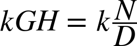
where N(s) is the numerator of the open-loop transfer function and D(s) is the denominator. Multiplying through by D, the characteristic equation can now be written as
Recall that those values s for which this equation is satisfied are the poles of the closed-loop transfer function and that all such values of s make up the root locus curves.
Now consider the two limiting cases of k → 0 and k → ∞. For k = 0, the characteristic equation reduces to D(s) = 0. In other words, in the limit of k = 0, the closed-loop transfer functions has poles when the denominator of the open-loop transfer function is zero: the poles of the open-loop and the closed-loop transfer functions coincide for k = 0. For the other limit, first divide through by k to obtain D(s)/k + N(s) = 0 and then let k → ∞; we are left with N(s) = 0. In this limit, the poles of the closed-loop transfer function coincide with the zeros of the open-loop transfer function (that is, those values of s for which the numerator N(s) of the open-loop transfer function vanishes.)
These observations lead to the following conclusion: the root locus curves begin at the poles of the open-loop transfer function for k = 0 and approach the zeros of the open-loop transfer function for k → ∞.
Root Locus or “Evans” Rules
Assume that the complete open-loop transfer function can be factored in the following way:

The transfer function has n poles and m zeros, and the condition n ≥ m ensures that it is proper.
We can now state[26] the following rules about the global appearance of a root locus diagram for nonnegative values of k. (These rules are also known as “Evans rules”, after W. R. Evans, who first formulated them.)
The root locus diagram is symmetrical with respect to the real axis.
There are n branches in the root locus diagram.
Every pole is a starting point (k = 0) of a branch. All branches begin at a pole.
Every zero is an endpoint (k → ∞) of a branch.
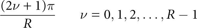
If there is an excess of poles over zeros, then the remaining R = n – m branches tend to infinity as k becomes large. (These branches end at the “zeros at infinity” of the transfer function.)
If the transfer function has R more poles than zeros, then the corresponding branches are asymptotic to straight lines as k → ∞. The asymptotes are at the following angles with the positive real axis:
All asymptotes intersect in a point on the real axis. The position σ0 of this intersection point is given by

If the transfer function has poles or zeros on the real axis, then those sections of the real axis that have an odd number of poles and zeros to their right will be part of one of the branches. Multiple poles or zeros are counted multiple times. (See examples later in this chapter!)
Different branches may intersect each other. Such points of intersection are called “singular points.” Singular points are values of s that satisfy the following equality:[27]

This is a necessary condition only—there may be solutions of this equation that correspond to negative values of k.
Branches intersecting on the real axis will depart from (or arrive on) the real axis at right angles to the real axis.
Employing these rules, a root locus diagram can be sketched by following this sequence of steps:
Plot the positions of the poles and zeros of the open-loop transfer function in the complex plane.
Identify those sections of the real axis that are part of one of the branches.
Plot the position where the asymptotes intersect.
Plot the asymptotes.
Plot the critical points (intersections of branches).
Angle and Magnitude Criteria
We can use the polar representation of complex numbers to derive two interesting conditions for a point s to lie on a root locus curve. Every complex number can be written in the polar form z = |z| eiϕ, where ϕ = arg z is the phase angle of z. Assume that the transfer function splits into factors as defined previously. We now use the polar representation of each factor (s – pj) and (s – zj):

to write the transfer function as

The characteristic equation requires that K(s)G(s)H(s) = −1. Using the polar representation of the transfer function just derived, we can write the characteristic equation as two separate equations for the magnitude and the phase angle. This leads to two conditions: the magnitude condition,
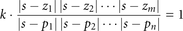
and the angle condition,

Because they must be satisfied simultaneously by any point s on a root locus curve, these two conditions can be used to determine whether a point belongs to one of the curves.[28]
Practical Issues
Root locus diagrams are a great way to develop a sense for the overall dynamic behavior of a system—although still fairly abstract, the map of roots and zeros provides more intuition than can a formula for the transfer function! At the same time, it is worth remembering that it is the dominant poles (those closest to the origin) that determine the behavior of the system. The global structure of the diagram is of less interest than the area near the origin.
The root locus diagram is an analytical technique. It requires an analytic expression for the transfer function of the plant or process, and it becomes more useful as the transfer functions become more complicated. If there is no good theoretical model of the system and one must employ a phenomenological descriptions obtained from experiments (see Chapter 8), then root locus diagrams are less necessary. In fact, as long as the transfer function is simple enough, one can work out the optimal positions of its dominant poles and zeros ahead of time and obtain “plug-in” rules for the controller gains (this is how the semi-analytical tuning methods in Chapter 9 work).
The root locus diagram is limited to displaying the movements of the poles and zeros as a single scalar parameter is varied. That is frequently not enough, since using a PI controller means that there are already two gain parameters to worry about. Employing a three-term controller or introducing a smoothing filter adds further adjustable parameters. Ultimately, this means creating a sequence of root locus diagrams, one for each value of the secondary parameter. (We’ll see an example later in this chapter.)
In most cases, root locus diagrams will be drawn with the aid of a computer. Specialized plotting programs exist[29] that take into account the special structure of the diagram and utilize the Evans rules to generate the plot. These programs usually require that the transfer function be specified explicitly as a strictly rational function.
Examples
In Chapter 20, we derived the transfer function for a simple lag:

This function describes systems, such as a heated vessel, that exhibit a particularly simple dynamic. If such a system undergoes a steplike change of its input, then its output will slowly approach its new steady-state value without oscillation or overshooting. (The temperature in a heated vessel increases steadily if the heat is turned on, and it decreases to the ambient temperature again if the heat is turned off.) Because the output does not respond immediately to the change in input, such systems are referred to as “simple lags.” The response to a step input of magnitude C that occurs at t = 0 is given by an exponential function in the time domain:
We have encountered this formula already as an approximate process model when looking for a phenomenological description of a system’s dynamic response (see Chapter 8 and Chapter 9).
Simple Lag with a P Controller
Consider a simple-lag system in combination with a proportional controller but without a return filter. In this case, we have
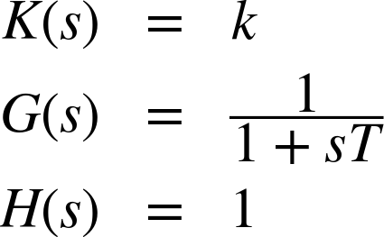
The open-loop transfer function is therefore
and the characteristic equation is

The open-loop transfer function has one pole (at s0 = –1/T) and no zeros, so we expect one asymptote at angle π with the positive real axis. In other words, the asymptote is parallel to the negative real axis.
In order to create a figure, we must assign a numerical value to the parameter T. Let’s set T = 1, which means that we measure time in units of T (see Figure 24-2).
The root locus diagram agrees with our expectations: there is only a single branch, it is aligned with the negative real axis, and it exhibits no oscillatory behavior. Increasing the controller gain k moves the pole to the left, starting from the pole at s0 = –1 and moving toward the “zero at infinity.” The part of the real axis to the left of the pole has “an odd number of poles (namely one) to its right” and is therefore part of the root locus curve (compare Rule 8).
A general problem with root locus diagrams is that the controller gain k is not shown. In Figure 24-2, we indicated several distinct values of k with symbols in the root locus diagram (top panel) and showed the corresponding step responses in the bottom panel. It is customary to use arrows to indicate the direction of increasing controller gain on each branch of a root locus diagram.

Simple Lag with a PI Controller
As discussed in Chapter 4, proportional control is generally insufficient to give good tracking performance because it will lead to “proportional droop.” This is evident in the step responses shown in Figure 24-2: even though increasing the gain increases the response time and reduces the tracking error, none of the curves manage to reach the input value in the steady state.
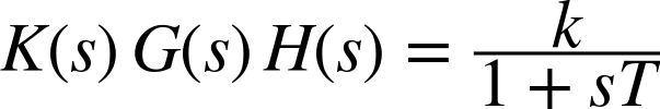
We therefore include an integral term in the controller, so that its transfer function now becomes
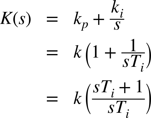
To construct a root locus diagram, we must use the alternate representation of the controller transfer function that involves the integral time constant Ti. Only this form of the transfer function allows us to factor out the variable parameter k, as is required.
For a PI controller and the simple-lag system considered previously, the characteristic equation is thus

This system has one zero (at z0 = –1/Ti) and two poles: one at the origin (p0 = 0) and the other at p1 = –1/T. Because there are two poles, we expect two branches; however, because the excess of poles over zeros is still R = 1, there is only a single asymptote, which is aligned with the negative real axis. The behavior in the time domain is a combination of two distinct contributions, one from each branch.
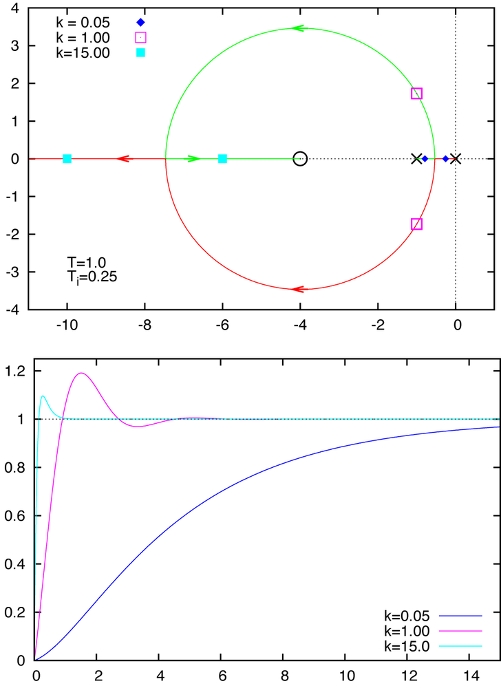
We should expect the diagram to look topologically different when the zero is between the two poles than when it is to the left of both—in other words, depending on whether (respectively) Ti > T or Ti < T. (This is a good example for the kind of consideration one must undertake when dealing with more than a single varying parameter in a root locus plot.) Figure 24-3 and Figure 24-4 show both cases.
If Ti > T then the zero lies between the two poles. The root locus curves are entirely real, and the step-response behavior is monotonic without oscillations. Observe again how the root locus curves include only those parts of the real axis with an odd number of poles and zeros to their right.
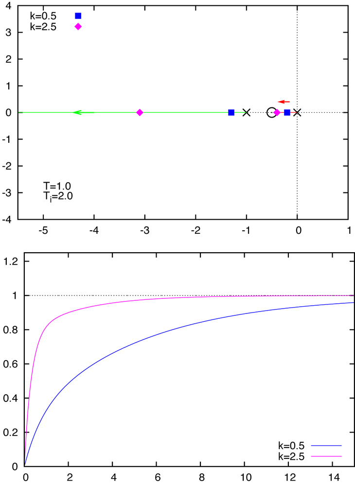
The step response for the lower value of the controller gain (k = 0.5) is dominated by the “slow” pole at –0.2, but in the step response for the higher value of the controller gain (k = 2.5) we can nicely see the effect of both poles. In this case, the amplitude of the slow pole at –0.4 is strongly reduced by its vicinity to the zero at –0.5, and so the initial response is dominated by the fast pole at –3.1. Only after the fast behavior has decayed does the response of the slow mode become apparent (and with a small amplitude).
Finally, if Ti < T then the root locus curves are no longer entirely confined to the real axis. When using values of k for which the poles have acquired an imaginary part, we find oscillatory behavior in the time domain. For this system, we find oscillatory behavior only for an intermediate range of controller gains: further increases in the controller gain lead again to nonoscillatory behavior, albeit with an initial overshoot.
[25] A note on terminology: I consider a root locus to be the position of a single solution of the characteristic equation. The root locus curve is the set of all such positions as the gain is varied.
[26] Derivations can be found, for example, in Modern Control Engineering by K. Ogata (2009).
[27] The general condition for a singular point is that dk/ds = 0, where k = – D(s)/N(s). If the transfer function factors completely, then this condition yields the formula given in the text.
[28] They can also be used to obtain further information about the appearance of a root locus diagram, such as the angles under which root locus curves enter or leave a pole or zero. For more information, see The Art of Control Engineering by K. Dutton, et al. (1997).
[29] Matlab, Scilab, and Octave all include routines for creating root locus diagrams.