Why do queues exist? They do not simply occur because resources are insufficient to handle incoming requests. Insufficient resources are the reason for exploding queues but not for queues in general.

Queues exist to smooth out variations. If customers arrived at (say) a bank in regular intervals and if each transaction took the same amount of time, then there would be no queues: we could schedule tellers to meet demand exactly. In fact, many automated manufacturing lines work in precisely this way. But if customers arrive randomly and if transactions can take up different amounts of time, then there will be moments when demand can (temporarily) not be met. This happens even if the tellers’ processing capacity is not less than the average arrival rate. There are only two ways to avoid such random accumulation of pending requests: scheduling arrivals periodically (thus reducing variation) or having an excess capacity of resources to handle requests (enough tellers to deal with anything). The first of these options is often not feasible, and the second is too expensive. Hence the need for queues and buffers.

What does this mean for queues from a control perspective? The most important point here is that it makes no sense to fix the queue length to one particular value: this would defeat the purpose of having a buffer in the first place! Instead, we usually want to restrict the length of the queue to some range, taking action (possibly drastic action) only if this range is violated. Keep in mind that it is often just as desirable to avoid an underflow of a buffer as it is to avoid an overflow: an empty buffer always means wasted resources (for example, tellers being idle).

We also need to ask what the overall goal of our control strategy is. In a physical environment, where a “buffer” is an actual device with a finite holding capacity (like a tank or an accumulating conveyor), we will mostly be concerned about avoiding overflows. But in more general situations, our goal will be to meet some quality-of-service expectation—and the length of the queue is not necessarily a good measure for the quality of service: a long queue that moves fast is more desirable than a short one that is stuck. In fact, the waiting time (or response time) will be a far better measure for our customer satisfaction. But the problem is a practical one: information about the waiting time may not be available! In order to base a system on waiting times, we must know the arrival time of each request, and this information is often not recorded. In contrast, the number of items pending is almost universally known. For this reason, it is desirable to have a strategy that works with only the length of the queue and without recourse to the actual waiting time.

Finally, a general concern when attempting to control queueing systems is that queues are slow and have difficult dynamics. If we only take action once a queue has become too long, it is—quite literally—too late. Not only has the queue already drifted from its target length, but we must now also process the accumulated backlog to bring the system back in line. The backlog requires additional resources to work through, which need to be decommissioned before the queue reaches its target length to prevent them from exhausting all the work and thereby underflowing the buffer. Buffers and queues are mechanisms for “memory” (in the sense of Chapter 3) and are hard to control. Therefore, early detection of change is essential. Note that this last requirement is in direct contradiction to the notion that we started with—namely, to let the length of a queue float!

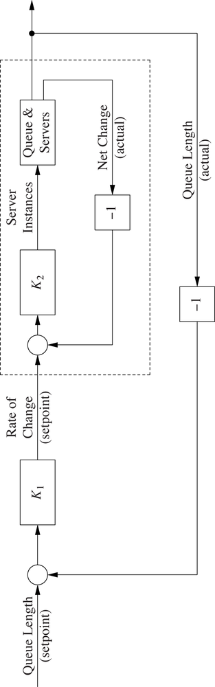
We will solve the challenges posed by the waiting queue problem by using a nested (or “cascaded”) control loop architecture (see Chapter 11). A fast-acting inner loop controls the actual plant, but the setpoint for the inner loop is provided by a controller in an outer loop.

Instead of controlling the length of the queue directly, in the present case the inner loop manages the rate of change of the length of the queue, adding or removing resources (servers) in order to keep the net change at the specified setpoint. The external loop, in contrast, will hold the overall length of the queue at the desired value without overwhelming the constraints of the buffer and without starving the downstream process. (See Figure 16-1.) The external loop provides the desired rate of change as the inner loop’s setpoint.

The internal loop will act quickly because it is monitoring the rate at which the queue length grows or shrinks. As soon as the queue begins to increase, the inner loop will add further servers to consume work items (and vice versa). The external loop will act more slowly, which is fine, since the setpoint for the external loop (namely, the desired length of the queue) will be changed only rarely.

To the external loop, the entire inner loop (shown by the dashed box in Figure 16-1) appears as a single component with exactly one input and output—in fact, the inner loop is the “plant,” which is controlled by the outer loop. Nevertheless, there are two controllers involved, both of which need to be tuned.

Consider the inner loop first. The actual plant here is quite similar to the server farm from Chapter 15. Again, the control input is the number of server instances that are active and ready to handle incoming requests. The difference now is that incoming requests that cannot be handled are queued instead of being discarded.

The inner controller is tuned like other systems with immediate-response dynamics (see Chapter 9). We know that each server can handle about 100 requests per time step, so the static gain factor is

Figure 16-1. A nested (cascaded) loop architecture. The outer loop provides the setpoint for the fast-acting inner loop.

Because there are no nontrivial dynamics, we can ignore the dynamic adjustments to the controller gain; however, we must still choose the contributions for each of the individual terms in the controller (see Chapter 14). Let’s use a PI controller with the following gains (including the static gain factor):

(The superscripts on the gain factors emphasize that these are the gains for the controller K₂ of the inner loop in Figure 16-1. Gains for the external controller K₁ will not be specially marked.)

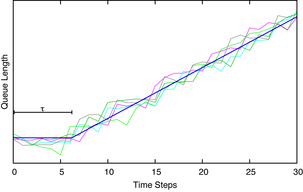
From this point on, the inner loop is simply treated as a black box: a component with a control input and output and with its own dynamics. As discussed in Chapter 8, we perform a step test on the inner loop to acquire the information needed to tune the external controller.

The results of the step test are shown in Figure 16-2.^[17] Since the inner loop is a queue, we should not be surprised that this is an accumulating process. Its ultimate rate of change is determined by the input to the inner loop. The delay can be found from the data: τ = 6.2. (A technical detail: before the step test, the queue should not be empty; if it is, then transients from the initial loading of the queue will obscure the steady-state behavior.)

Results from the step test can now be employed to find parameters for the controller in the outer loop, using entries for the AMIGO method for accumulating processes from Table 9-1. The resulting gains are (approximately)

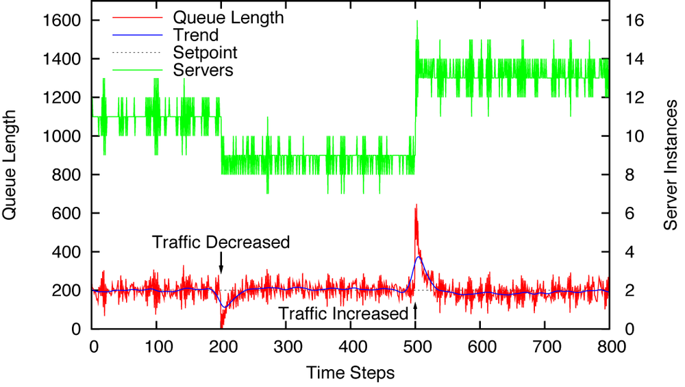
Typical results when using a two-term (PI) controller are shown in Figure 16-3. The setpoint is held constant at r = 200, and the intensity of incoming traffic changes twice over the course of the experiment. (The final traffic is about 20 percent higher than the original one.) We see that the external controller is able to maintain the setpoint in the steady state but that the system does not respond well to changes. As the traffic intensity decreases, the number of server instances is not reduced quickly enough to prevent the queue from running empty for about 50 time steps. Much worse is the behavior as the traffic intensity suddenly increases: by the time enough server instances are online to handle the new load, the queue has overshot the setpoint by a factor of almost 7!

Figure 16-2. Results of step tests performed on the inner loop.

Figure 16-3. Behavior of the outer loop under PI control with k_p = 0.06 and k_i = 0.001.

The reason for the poor performance is clear: the external controller does not respond adequately to persistent deviations of the queue length from the selected setpoint. However, we cannot increase the integral gain without bringing about violent control oscillations. But there is another term in the proverbial “three-term” or PID controller that responds to changes in the tracking error: the derivative term.

We have not used derivative control much (or at all) in this book, given that the derivative term is susceptible to noise (see Chapter 4) and that most of the systems we have considered are noisy. In this example the queue length is also noisy, so why do we believe that derivative control might be applicable now when it wasn’t before? The reason is that we have decoupled the time scales. Because fast response to high-frequency noise is handled by the inner loop, the external loop can respond more slowly. In particular, we can apply a smoothing filter to remove most of the noise and then use derivative action to bring about a quicker response to changes in the queue length.

Figure 16-4 is typical for the best behavior that can be obtained in this way. The derivative action is filtered using a recursive filter with α = 0.15 (see Chapter 10), and the controller gains are adjusted manually from the settings suggested by the AMIGO tuning method. The gains used were

The performance is much improved over the behavior without derivative action. The interval where the queue is running empty as the traffic intensity decreases has been almost eliminated, and the overshoot in response to the increase in traffic has been reduced by more than half.

Finally, observe that the number of server instances changes more frequently than before. This is a consequence of the derivative term, which tends to enhance high-frequency noise. An excessive amount of control actions is usually undesirable, so we may want to insert a smoothing filter between the external controller and the inner loop. Such a filter will stabilize the setpoint experienced by the inner loop. Figure 16-5 shows what happens after a recursive filter with α = 0.5 has been added: the number of server instances fluctuates less, yet the behavior of the queue length is hardly affected at all. Notice that we can apply only a moderate amount of smoothing. As soon as we begin to make α smaller (thereby enhancing the effect of the filter), the queue length begins to drift.

Figure 16-4. Behavior of the outer loop when a derivative term is included in the K₁ controller.

Figure 16-5. Similar to Figure 16-4, but now an additional smoothing filter has been inserted between the external controller and the inner loop.

The nested loop arrangement described here involves two controllers, one each for the outer and the inner loop. For the present solution, we have chosen to use controllers of the PID (or PI) type for both. The resulting performance may be good enough, but it is worth considering alternatives.

The inner loop is suffering from the defect—encountered already in Chapter 15—that you can’t have “half a server.” If the number of servers required to maintain a particular setpoint is not a whole integer, then the system will end up oscillating rapidly between the two neighboring states. To avoid this artifact, we might want to consider a controller, like the one discussed in Chapter 15, that knows about the integer constraint and switches the number of server instances less frequently. Such a controller will typically exhibit some form of hysteresis in that the number of servers is not changed unless the reasons for a change become sufficiently strong. Such an arrangement will reduce the number of control actions, but it will also decrease the system’s tracking accuracy because hysteresis will prevent the system from responding quickly to changes in control input. It will be an engineering decision to balance these requirements.

The controller in the external loop maintains the overall queue length. In the current arrangement, the controller attempts to keep the queue at one specific setpoint value, but it may be more appropriate to keep the queue within a particular range. This would require a controller that generates little (or no) control action if the tracking error is small but that generates a disproportionately large corrective action whenever the tracking error leaves the desired range. One could try an “error-square” controller (see Chapter 10) or invent a special-purpose controller for this purpose. Whether a special-purpose controller is necessary for a particular application is, again, an engineering decision. One argument generally favoring PID controllers is their simplicity and the relatively small number of adjustable parameters they require.

The simulation for the queueing system makes use of the AbstractServerPool base class that was introduced in Chapter 15. (Code discussed previously is not reproduced here.) The main difference between the QueueingServerPool used here and the ServerPool used in Chapter 15 is that, in the present case, the new load is added to the existing queue instead of replacing it.

class QueueingServerPool( AbstractServerPool ):
    def work( self, u ):
        load = self.load()      # additions to the queue
        self.queue += load      # new load is added to old load

        completed = AbstractServerPool.work( self, u )

        return load - completed # net change in queue length

Recall that the AbstractServerPool does not model individual requests. Instead, we specify two functions to place an aggregate “load” onto the queue and one that simulates the “work” done by the servers. This implies that no information regarding individual requests (such as their arrival time or age) is available. Hence the implementation of the QueueingServerPool just described reports only the net change in queue length as process output.

The QueueingServerPool, when used in a closed-loop arrangement with a PI controller, forms the inner loop of the overall architecture (compare Figure 16-1). As far as the outer loop is concerned, the entire inner loop is just another component: it has a control input and a control output. We therefore model the inner loop as a subclass of the general Component abstraction from the simulation framework:

class InnerLoop( fb.Component ):
    def __init__( self, kp, ki, loader ):
        k = 1/100.

        self.c = fb.PidController( kp*k, ki*k )
        self.p = QueueingServerPool( 0, consume_queue, loader )

        self.y = 0

    def work( self, u ):
        e = u - self.y       # u is setpoint from outer loop
        e = -e               # inverted dynamics
        v = self.c.work( e )
        self.y = self.p.work( v ) # y is net change
        return self.p.queue

    def monitoring( self ):
        return "%s %d" % ( self.p.monitoring(), self.y )

To run the simulations, we need a setpoint that changes over time as well as a load function that models varying intensity of request traffic. (The load_queue() function must use a global variable to keep track of the current time step.)

def load_queue():
    global global_time
    global_time += 1

    if global_time > 2500:
        return random.gauss( 1200, 5 )

    if global_time > 2200:
        return random.gauss( 800, 5 )

    return random.gauss( 1000, 5 )


def setpoint( t ):
    return 200

    if t < 2000:
        return 100
    elif t < 3000:
        return 125
    else:
        return 25

With all these definitions now in place, we can give the code for the simulation used to produce the data shown in Figure 16-4. (Notice the additional filter inserted as “actuator” between the external controller and the inner loop.)

import feedback as fb

fb.DT = 1

global_time = 0 # To communicate with load_queue functions

p = InnerLoop(0.5, 0.25, load_queue) # "plant" for outer loop
c = fb.AdvController( 0.35, 0.0025, 4.5, smooth=0.15 )

fb.closed_loop( setpoint, c, p,
                actuator=fb.RecursiveFilter(0.5) )