
Chapter 10
Flowsheet Analysis for Pollution Prevention
10.1 Introduction
The environmental performance of a process flowsheet depends on both the performance of the individual unit operations that make up the flowsheet and on the level to which the process streams have been networked and integrated. While Chapter 9 describes methods for improving the performance of individual unit operations, this chapter examines methods for assessing and improving the degree to which the unit operations are integrated. Specifically, Section 10.2 examines process energy integration and Section 10.3 examines process mass integration. The methods presented in these sections, and the case study presented in Section 10.4, demonstrate that improved process integration can lead to improvements in overall mass and energy efficiency.
Before examining process integration in detail, however, it is useful to review the methods that exist for sytematically assessing and improving the environmental performance of process designs. A number of such methods are available. Some are analogous to Hazard and Operability (HAZ-OP) Analyses (e.g., see Crowl and Louvar, 1990).
Section 9.7 briefly describes how a Haz-Op analysis is performed; to summarize, the potential hazard associated with each process stream is evaluated qualitatively (and sometimes quantitatively) by systematically considering possible deviations in the stream. Table 10.1-1 gives the guide words and examples of deviations used in HAZ-OP analysis. Each guide word is applied to each relevant stream characteristic, the possible causes of the deviation are listed, and the consequences of the deviation are determined. Finally, the action(s) required to prevent the occurrence of the deviation are determined.
Table 10.1-1 Guide Words and Deviations in HAZ-OP Analysis.
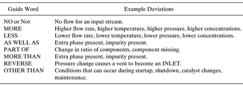
For a single pipeline taking fluid from one storage tank to another, there may be several possible deviations, such as:
• no flow
• more flow
• more pressure
• more temperature
• less flow
• less temperature
• high concentration of a particular component
• presence of undesirable compounds
Note that each deviation may have more than one possible cause so that this set of deviations would be associated with dozens of possible causes. It would be difficult to consider all the deviations and their consequences without a structured system for analyzing the flowsheet. A similar analysis framework has been employed in a series of case studies to identify environmental improvements in process flowsheets (DuPont, 1993). In these case studies, a series of systematic questions are raised concerning each process stream or group of unit processes. Typical questions include:
• What changes in operating procedures might reduce wastes?
• Would changes in raw materials or process chemistry be effective?
• Would improvements in process control be effective?
Process alternatives, such as those defined in Chapter 9, can be identified, and in this way the environmental improvement opportunities for the entire flow-sheet can be systematically examined. (See, for example, the cases from the DuPont report described by Allen and Rosselot, 1997.)
Other methods for systematically examining environmental improvement opportunities for flowsheets have been developed based on the hierarchical design methodologies developed by Douglas (1992). The hierarchical levels are shown in Table 10.1-2. Note that Level 1 in this table applies only to processes that are being designed, not to existing processes. The hierarchy is organized so that decisions that affect waste and emission generation at each level limit the decisions in the levels below it.
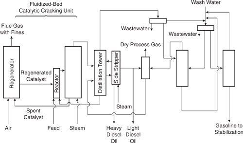
As an example of the use of hierarchical analysis procedures, consider a case study drawn from the AMOCO/US EPA Pollution Prevention Project at AMOCO’s refinery in Yorktown, Virginia (Rossiter and Klee, 1995). In this example (adapted from Allen and Rosselot, Pollution Prevention for Chemical Processes, © 1997. This material is used by permission of John Wiley & Sons, Inc.), the flowsheet of a fluidized-bed catalytic cracking unit (FCCU) is evaluated for pollution prevention options. A flowsheet of the unit is shown in Figure 10.1-1.
Beginning with Level 2 of the hierarchy listed in Table 10.1-2 (input-output structure), the following pollution prevention strategies were generated:
1) Improve quality of the feed to eliminate or reduce the need for the vapor line washing system shown in the upper right-hand corner of Figure 10.1-1.
2) Reduce steam consumption in the reactor so that there is less condensate to remove from the distillation system.
3) Within the catalyst regeneration system, the loss of fines (upper left hand corner of Figure 10.1-1) is partly a function of the air input rate. A reduction in air flow (e.g., by using oxygen enrichment) is a possible means of reducing the discharge of fines.
Two ideas were generated during review of the recycle structure (level 3):
1) The reactor uses 26,000 lb/hr of steam. This is provided from the utility steam system. If this could be replaced with steam generated from process water, the liquid effluent from the unit would be reduced. Volatile hydrocarbons contained in the recycled steam would be returned directly to the process. Catalyst regeneration consumes more than 11,000 lb/hr of steam. It may be possible to satisfy this duty with “dirty steam” as well, since the hydrocarbon content would be incinerated with the coke in the regenerator.
Table 10.1-2 Levels for Hierarchical Analysis for Pollution Prevention (Adapted from Douglas, 1992).

Figure 10.1-1 Process flow diagram of a fluidized-bed catalytic cracking unit.
2) Used wash water is collected at several points and then purged from the process. If it could be recovered and recycled instead, or if recycled water from other sources could be used for washing in place of fresh water, fresh water usage and wastewater generation could both be reduced by about 10,500 lb/hr.
Three options were identified for separation systems (level 4):
1) Replace heating done by direct contacting with steam by heating with reboilers.
2) Place additional oil-water separators downstream of existing condensate collection points and recover hydrocarbons.
3) Improve gas-solid separation downstream of the regenerator to eliminate loss of catalyst fines. This might simply require better cyclone and/or ductwork design, or electrostatic precipitation.
These first four levels of the design hierarchy lead us to the types of process improvements described in Chapter 9—improvements in the reactor and improvements in the separation system. As Table 10.2-1 notes, the next step in the design process is to identify opportunities for process integration. This is the main topic of this chapter and the next several sections describe methods for process energy integration and methods for identifying process waste recycling and reuse opportunities.
10.2 Process Energy Integration
Process streams frequently need to be heated, often to achieve the correct conditions for a desired reaction or to achieve separation of materials. Heating of process streams is generally done in furnaces or by contacting process streams with steam or other energy carrier fluids. No matter whether it is done in a furnace or using steam generated in a boiler, heating a process stream generally requires combustion of fuels, adding expense and environmental impacts to a process.
Process streams also frequently need to be cooled. This cooling is frequently done with cooling water which is circulated throughout the process. Cooling towers are used to keep cooling water temperatures at steady state values, but operating these cooling towers consumes energy and causes the loss of water through evaporation, adding expense and environmental impacts to a process.
The idea behind process heat or process energy integration is to use the heat from streams that need to be cooled for heating streams that need their temperature raised. Heat transfer between streams in a process prevents pollution by reducing the need for fuels and for cooling tower operation. Process heat integration is generally done using an analysis referred to as heat exchange network (HEN) synthesis. In heat exchange network synthesis, all of the heating and cooling requirements for a process are systematically examined to determine the extent to which streams that need to have their temperature raised can be heated by streams that need to be cooled. Heat integration is discussed in engineering undergraduate courses and detailed descriptions of HEN synthesis are available in most modern textbooks of chemical process design (e.g., Douglas, 1988). A simple example is described here in order to refresh readers on the basic concepts.
Figure 10.2-1 shows a heat balance diagram for a stream that needs to be heated from 50°C to 200°C and a stream that needs to be cooled from 200°C to 30°C. For the sake of simplicity, both streams in this example have a heat capacity of 1 kJ/(kg-°C). The stream that needs to be cooled has a flow rate of 1 kg/s and the stream that needs to be heated has a flow rate of 2 kg/s. Heating and cooling utilities could be applied to the two streams separately, as shown in Figure 10.2-2. However, the requirements for heating and cooling utilities are less if heat exchange between the two streams occurs.
Figure 10.2-1 Heat balance diagram for a hot process stream and a cold process stream.
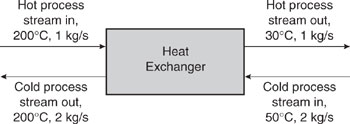
There are two fundamental thermodynamic constraints to heat transfer. One is that the quantity of heat absorbed by the cold stream (the stream that needs to be heated) is equal to the quantity of heat lost by the hot stream (the stream that needs to be cooled). The other constraint is that heat flows from higher temperature streams to lower temperature streams.
One particularly useful way to graphically depict the streams to be heated and cooled in a flowsheet is called a “pinch” diagram. This diagram can be used to determine the extent to which heat transfer is possible and also to determine which hot streams should be paired with which cold streams. Heat transferred to and from the streams is on the y-axis in a pinch diagram and temperature is on the x-axis. Hot streams are represented as lines that slope downward and to the left, while cold streams are represented by lines that slope upwards and to the right. The hot and cold streams of Figure 10.2-1 are depicted in the pinch diagram of Figure 10.2-3.
Figure 10.2-2 Heating and cooling requirements before heat integration.
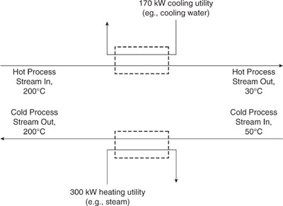
Figure 10.2-3 Hot stream and cold stream load line diagram for heat exchange network synthesis.

Note that the vector representing the cold stream (that needs to be heated) begins at a temperature of 50°C. It ends at a temperature of 200°C and at an enthalpy 300 kW higher than it started. Similarly, the hot stream (that needs to be cooled) begins at a temperature of 200°C and ends at a temperature of 30°C, and an enthalpy 170 kW lower than it started.
The enthalpy units in a pinch diagram, such as Figure 10.2-3, are relative. Be-cause of this, both hot and cold stream lines are free to move vertically. However, because of the thermodynamic constraints, heat transfer between the streams can take place only in regions where the hot stream lies to the right of the cold stream (i.e., where the hot stream is at a higher temperature than the cold stream—in Figure 10.2-3, the region between the dashed lines that intersect the energy axis at 100 and 240 kW). The maximum theoretical heat transfer between the streams occurs when the two streams touch but do not cross. This point is called the thermal pinch. This theoretical maximum is not possible in practice because an infinitely large heat exchanger would be required to effect heat exchange at the point where the temperature difference between the streams goes to zero.
As the lines move apart, the region where the hot stream lies to the right of the cold stream becomes smaller and the amount of heat transferred between the streams decreases. As a result, the utility requirements for heating and cooling the streams to their target temperatures increase. In contrast, the heat exchanger for transferring heat from the hot stream to the cold stream gets smaller as the lines move apart. Thus, there is an optimum temperature driving force where total annualized costs (operating, or utility, costs plus capital costs of the heat exchanger) are minimized.
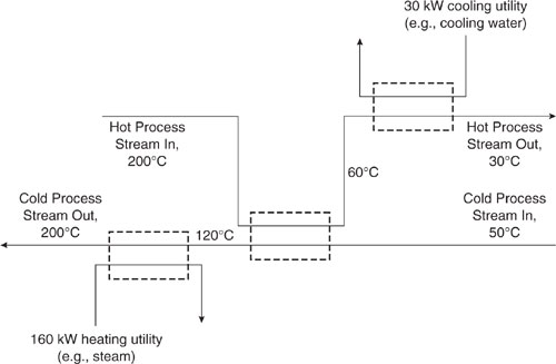
If the optimum temperature difference is 10°C, then the pinch diagram of Figure 10.2-3 shows the optimum heat transfer between the two streams to be 240 - kW 100 kW = 140 kW. The diagram also shows that, under these conditions, the cold stream is heated from 50°C to 120°C in the exchanger and the hot stream is cooled from 200 C to 60 C. A diagram of the heat exchange network is given in Figure 10.2-4. Comparison of Figure 10.2-4 with Figure 10.2-2 shows that heat integration results in a substantial decrease in the utilities needed to heat and cool the two streams to their target temperatures.
This simple example of process heat integration illustrates a basic concept— that exchange of energy between process streams that need to be heated and process streams that need to be cooled (process energy integration) can reduce overall energy demand for a process. More complete treatments of HEN synthesis are available in standard chemical process design texts and this chapter will not describe these methods in detail. Rather the focus of the remainder of this chapter will be on a topic analogous to HEN synthesis, but one that is not normally addressed in chemical process designs—process mass integration and mass exchange network synthesis.
Figure 10.2-4 Heating and cooling requirements after heat integration.
10.3 Process Mass Integration
Just as heat integration is the use of heat that would otherwise be wasted, mass integration is the use of materials that would otherwise be wasted. Three tools for determining process configurations that result in mass integration are described in this section. The first tool, source-sink mapping, is the most visual and intuitive of the three. Next, a strategy for determining optimum mixing, segregation, and recycle strategies is described. Finally, mass exchange network synthesis, which is the mass integration analogue for heat exchange network synthesis, is described.
10.3.1 Source-Sink Mapping
Source-sink mapping is used to determine whether waste streams can be used as feedstocks. It is the first quantitative tool for mass integration discussed in this chapter because it is one of the simplest and most visual tools for identifying candidate streams for mass integration.
The first step in creating a source-sink diagram is to identify the sources and sinks of the material for which integration is desired. For example, if water integration is desired, then wastewater streams (the “sources” of water) are identified. The processes that require water (the “sinks” of water) must also be identified. The flow rates of the sources and sinks must be known, keeping in mind that many sinks can accept a range of flow rates. Contaminants that are present in the source streams and that pose a potential problem for the sinks must be identified, and the tolerance of each sink for these contaminants must be known. Some processes require very pure feed, in which case using waste streams that contain the feed material as well as some contaminants is infeasible. However, many processes can make use of material that contains impurities, and some sinks have extremely liberal tolerances. The final piece of information that must be known before constructing a source-sink diagram is the concentration of contaminants that were identified as being potentially significant problems for the sinks.
Once all of these parameters are known, the source-sink diagram can be drawn. If only one contaminant is a concern, the diagram is two-dimensional, with source and sink flow rates plotted on the y-axis and contaminant concentration plotted on the x-axis. Each sink is represented by an area corresponding to its upper and lower limits of tolerance for flow rate and contamination, and each source is represented by a point.
As an example of the construction of a source-sink diagram, consider the sources and sinks described in Table 10.3-1. The material for which integration is sought (assume, for the moment that this is water) is available at the flow rate specified and the contaminant of concern is X. Figure 10.3-1 shows a source-sink diagram for the streams described in this table. Sources A, B, and C are shown as points in Figure 10.3-1 (because the flow rate and contaminant concentrations are point values), while sinks 1 and 2 are shown as shaded areas (because the flow rate needed and acceptable contaminant concentrations are ranges of values).
Table 10.3-1 Example Stream Data for Source-Sink Diagram.

An initial examination of Figure 10.3-1 indicates that stream C could be used to partially satisfy the water demand for stream 1, since stream C’s contaminant concentration falls within the range allowed for stream 1. No other direct reuse opportunities are available; however, stream A has a concentration that is not too far above the maximum allowable contaminant concentration for stream 1. Would it be possible to blend streams A and C and satisfy the contaminant constraint for stream 1?
Source streams whose concentration of contaminants is too high for feeding to any sinks (such as A) can be combined with low-concentration sources (such as C) to lower their concentration. In Figure 10.3-1, a point representing a combination of sources A and C is depicted. The flow rate of the combined streams is simply the sum of the flow rates of the individual streams, and the concentration of compound X in the combined stream is the weighted average of the concentration in streams A and C,

Figure 10.3-1 Source-sink diagram for the streams of Table 10.3-1.
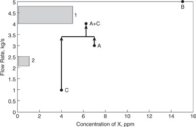
Note that this point representing the combined stream A-C has a flow rate within the acceptable range for sink 1, but its concentration of contaminant X is too high to allow the combined stream to be used directly in sink 1. In other words, streams A and C cannot be combined and used as the sole feedstock for sink 1.
To lower the concentration to within acceptable limits, uncontaminated material (fresh water with 0 concentration of X) must be used in addition to sources A and C. The most uncontaminated material that can be added to the stream to lower the concentration of X (while still using all of streams A and C to minimize water treatment requirements) is 0.8 kg/s, because more than that will create a stream with a larger flow rate than the upper bound allowed by sink 1. If 0.8 kg/s of uncontaminated material is added to streams A and C, the concentration of X in the combined stream will be
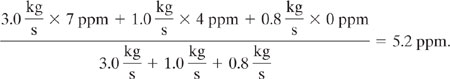
This concentration is still higher than the limit allowed by sink 1. To lower the concentration further without exceeding the limit on flow rate, only a portion of source A can be used. For example, if 2.8 kg/s of source A, all of source C, and 1.0 kg/s of uncontaminated material were combined, the resulting stream could be fed to sink 1. This is shown graphically in Figure 10.3-2.
The following example shows an application of source-sink mapping for a process that manufactures acrylonitrile.
Example 10.3-1 Source-Sink Mapping for Acrylonitrile Production.
Background
A simplified flowsheet for the production of acrylonitrile is given in Figure 10.3-3 (El-Halwagi, 1997). The chemistry of this process was described in Chapter 8. Oxygen, ammonia, and propylene are reacted to form a gaseous stream containing the product, ammonia, and water. This stream is sent to a condenser where most of the water is removed in a stream that is sent to treatment.
The gaseous stream from the condenser is then sent to a scrubber where it is washed into a liquid stream that is fed to the decanter. Off-gases from the scrubber contain a negligible amount of water, acrylonitrile, and ammonia.
Figure 10.3-2 Source-sink diagram for Table 10.3-1, with sources and fresh feed combined to coordinate with a sink.

Figure 10.3-3 Flowsheet for production of acrylonitrile (AN).
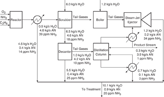
The output of the scrubber is a mixture of water, acrylonitrile, and ammonia. This stream is sent to a decanter, where an aqueous layer and an organic layer (containing most of the acrylonitrile) form. All but 1 kg/s of the aqueous layer is sent to treatment, and the non-aqueous layer along with the remaining aqueous layer (1 kg/s) is sent to a distillation column in order to further purify it. A negligible amount of water is dissolved in the acrylonitrile layer, but 0.068 mass fraction acrylonitrile is found in the aqueous layer. Both the aqueous layer and the acrylonitrile layer from the decanter contain ammonia, with the concentration in the aqueous layer higher by a factor of 4.3. The entire non-aqueous layer and some of the aqueous layer from the decanter is sent to the distillation column for further purification of acrylonitrile. As long as the feed to the distillation column is between 15 and 25 ppm NH3 and between 75% and 85% by mass acrylonitrile, the bottoms stream from the column does not change. This stream is sent to treatment.
The distillation column is operated at a vacuum, which is supplied by a steam-jet ejector. Some of the material in the distillation column is carried off in the ejectate stream, including 0.2 kg/s acrylonitrile. No appreciable quantity of water is pulled off in the ejectate, and the concentration of ammonia in the ejectate stream is a factor of 34 higher than the concentration of ammonia in the acrylonitrile product stream from the top of the distillation column. The ejectate stream is sent to treatment.
In this simplified example, integration of water and acrylonitrile is sought and the only contaminant of concern is ammonia. The liquid feed to the scrubber must be between 5.8 and 6.2 kg/s, and can consist of water or a mixture of water and acrylonitrile. The concentration of ammonia in the feed to the scrubber must not exceed 10 ppm. In contrast, the feed to the boiler cannot contain any ammonia or acrylonitrile and is required to be 1.2 kg/s.
Problem Statement
a. How many sources of water are there in the process? How many sinks?
b. Draw a source-sink diagram for the process, with total flow rate (water plus acrylonitrile) on the y-axis and ammonia concentration on the x-axis.
c. What wastewater streams can be used as feed for the scrubber?
d. What wastewater streams can be in the boiler?
e. If the amount of acrylonitrile fed to the scrubber is to be maximized, what will be the flows of wastewater from each wastewater stream to the scrubber?
f. Draw a diagram that shows the new flowsheet. If these flows are put into place, what is the flow rate of water and acrylonitrile and the concentration of ammonia in all of the streams downstream of the scrubber?
g. How does the product stream differ from the original configuration?
h. How does the quantity of fresh water feed differ?
i. How does the total stream sent to wastewater treatment differ?
Solution:
a. The sources of wastewater and waste acrylonitrile are the condenser, the decanter, the distillation column, and the ejectate. Sinks are the scrubber and the boiler.
b. Figure 10.3-4 shows a source-sink diagram for this process. Note that none of the wastewater streams can be used as feed for the boiler because they all contain acrylonitrile or ammonia or both.
Figure 10.3-4 Source-sink diagram for acrylonitrile process (AN acrylonitrile).
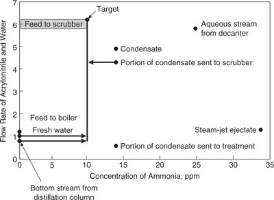
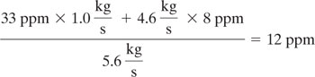
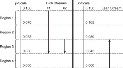
c. Examination of the source-sink diagram reveals that the bottom stream from the distillation column and the wastewater stream from the condenser are likely candidates for feed to the scrubber. In fact, because the bottom stream from the distillation column contains no ammonia and has the highest mass fraction of acrylonitrile of any waste stream, that entire stream should be fed to the scrubber. The maximum amount of acrylonitrile in the wastewater streams from the condenser is returned to the process when the scrubber is fed its maximum amount of feed (6.2 kg/s) at the maximum concentration of ammonia (10 ppm). If x is the flow rate of the condensate stream sent to the scrubber and y is the flow rate of fresh water to the scrubber, then balances for water and ammonia flow give:
![]()

Solving for x and y gives x 4.4 kg/s and y 1.0 kg/s. In other words, 4.4 kg/s of the condenser wastewater stream (consisting of 4.0 kg/s water and 0.4 kg/s acrylonitrile) and all of the bottom stream from the distillation column along with 1 kg/s of fresh water can be used as scrubber feed. This is shown in the source-sink diagram of Figure 10.3-4.
To find the characteristics of each stream downstream of the scrubber, which are now different from those shown in Figure 10.3-3 (because the feed to the scrubber is different), do a mass balance of water, acrylonitrile, and ammonia over the scrubber. A diagram for the mass balance is shown in Figure 10.3-5.
The flow rate of water leaving the scrubber is
![]()
and the flow rate of acrylonitrile leaving the scrubber is
![]()
The concentration of ammonia in the stream leaving the scrubber is found using the equation

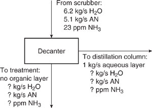
Next, mass balances are performed around the decanter, pictured in Figure 10.3-6, to find its outlet stream characteristics. Keep in mind that in the decanter, the stream from the scrubber forms two layers: an aqueous layer containing some acrylonitrile and ammonia, and an organic layer containing a negligible amount of water and some ammonia. All of the organic layer and 1 kg/s of the aqueous layer go to the distillation column and the remaining portion of the aqueous layer goes to wastewater treatment.
Figure 10.3-5 Mass balance diagram for scrubber in acrylonitrile process (AN acrylonitrile).
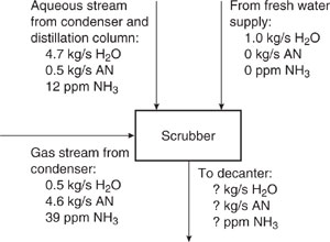
Figure 10.3-6 Mass balance diagram for decanter in acrylonitrile process (AN acrylonitrile).
The relationship for acrylonitrile in the aqueous layer can be used to find the flow rate of water to the distillation column, as follows:
![]()
where z is the flow rate of the water in the aqueous layer sent to the distillation column. Solving gives
![]()
A water mass balance around the decanter gives the flow rate of water in the stream sent to treatment:
![]()
The flow rate of acrylonitrile in the stream sent to treatment is given by
![]()
From a mass balance for acrylonitrile, one can find the acrylonitrile being sent to the distillation column:
![]()
The concentration of ammonia in the streams leaving the decanter depends on the flow rates of the aqueous layer and organic layer, rather than on the flow rates of water and acrylonitrile leaving the decanter. Therefore, the next step is to find the flow rates of the aqueous layer and the organic layer. The total flow rate of the aqueous layer is equal to the total flow rate sent to treatment plus 1 kg/s that is sent to the distillation column, or
![]()
and the total flow rate of the organic layer is 4.7 kg/s. Now, if x is the concentration in ppm of ammonia in the aqueous layer and y is the concentration in ppm of ammonia in the organic layer, then a mass balance for ammonia around the decanter gives
![]()
It is given that
![]()
and solving for x and y gives y = 8 ppm and x = 33 ppm. The overall concentration of ammonia in the stream sent to the distillation column is
Now, mass balances can be performed around the distillation column of Figure 10.3-7 in order to find the characteristics of the product stream and the steam-jet ejectate.
The bottoms stream is the same as before and there is no water carried away in the steam-jet ejectate, so a mass balance for water gives the water in the product stream, as follows:
![]()
The amount of acrylonitrile in the steam-jet ejectate stream is given, and again, the bottoms from the distillation column do not change, so the amount of acrylonitrile in the product stream is given by
![]()
Next, a mass balance for ammonia, plus the relationship for ammonia concentrations in the product stream and the steam-jet ejectate, are used to find the concentration of ammonia in those streams. If x is the concentration of ammonia in ppm in the product stream and y is the concentration of ammonia in ppm in the steam-jet ejectate, then
![]()
![]()
Solving gives x = 2 ppm ammonia and y = 50 ppm ammonia.
Figure 10.3-7 Mass balance diagram for the distillation column in the acrylonitrile process (AN acrylonitrile).

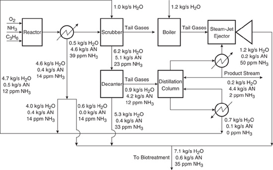
The final flowsheet is given in Figure 10.3-8, and the differences between the outputs (wastewater and product stream) of the original configuration and the configuration with wastewater reuse are given in Table 10.3-2. The requirement for fresh water feed is 30% of the original process, and the flow rate of material sent to treatment is 60% of the original process. The mass fraction of acrylonitrile in the stream sent to treatment is lower than before by 15%, but the ammonia concentration in the stream sent to treatment is nearly a factor of two larger. Also, the concentration of ammonia in the product stream is twice what it was before wastewater reuse. More important than any of these changes, however, may be the increase in the production of acrylonitrile from 3.9 kg/s to 4.4 kg/s. With a market value of $0.60/kg and 350 days per year of production, this increase in product is worth $9,000,000 a year.
Table 10.3-2 Outputs from the Production of Acrylonitrile Before and After Wastewater Reuse.

Figure 10.3-8 Flowsheet for acrylonitrile (AN) after identifying opportunity for water integration using source-sink mapping.
10.3.2 Optimizing Strategies for Segregation, Mixing, and Recycle of Streams
The source sink mapping described in the acrylonitrile example was a relatively simple example with just a few sources and sinks. As the processes to be analyzed become more complex and the number of sources and sinks increase, mathematical optimization techniques, coupled with process simulation packages, are generally employed to identify opportunities for recycle, segregation, and mixing of streams. The linear and non-linear mathematical programming techniques employed in these optimizations are beyond the scope of this text; however, the following example of source-sink matching for a chloroethane facility begins to illustrate the potential complexity of the problems that can be encountered.
Example 10.3-2 Source-Sink Mapping for Chloroethane Production.
Figure 10.3-9 is a flow diagram of a process for producing chloroethane. In this process, ethanol and hydrogen chloride are reacted in the presence of a catalyst to create chloroethane. The reaction is written as follows:
C2H5OH→C2H5Cl + H2O
Chloroethanol is also created in the reactor as an unwanted byproduct.
Two phases leave the reactor: an aqueous phase that is sent to wastewater treatment, and a gaseous phase that contains the product. The gaseous phase leaving the reactor contains unreacted ethanol and hydrogen chloride as well as chloroethane and chloroethanol and is sent through two scrubbers in sequence in order to purify it enough for finishing steps and eventual sale. The aqueous streams from the two scrubbers are mixed and recycled back to the reactor because a fraction of the chloroethanol they contain can be converted into chloroethane (the desired product) via a reduction reaction whose rate is directly proportional to the concentration of chloroethanol in the aqueous stream entering the reactor. This conversion of chloroethanol to chloroethane is the key to minimizing the overall generation of chloroethanol in the process. Configuring the process streams so that the concentration of chloroethanol in the aqueous stream fed to the reactor results in as much destruction of chloroethanol as possible results in the minimum generation of this pollutant.
Figure 10.3-9 Process flow sheet for original configuration of chloroethane process. Concentrations of chloroethanol and total flow rates are given for the stream sent to wastewater treatment as well as the product stream. Flow rates of fresh water to scrubbers are also given.
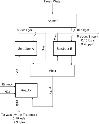
The goal of the analysis presented in this example is to determine how streams should be segregated, mixed, and recycled so that the net generation of chloroethanol is minimized. To provide a visual aid for the analysis, the process flowsheet can be redrawn as shown in Figure 10.3-10. This figure shows that each aqueous stream from each process unit can be split and sent to either wastewater treatment, sent back to the process unit from which it originated, or sent to one of the other process units. Mixers are located just prior to each process unit, and separators are located on the stream exiting each process unit. In the solution, the quantity of each stream that is sent to each option is determined. Note that the gaseous stream from the reactor must proceed through scrubber A, then through scrubber B.
Note that the process units have been assigned numbers. The reactor is unit number one, scrubber A is unit number two, scrubber B is unit number three, waste-water treatment is unit number four, and the source supplying fresh water is unit number five. The concentration of chloroethanol in ppm in the aqueous streams are given as x, and the concentration of chloroethanol in ppm in the gaseous streams is called y. Aqueous stream flow rates in kg/s are given as L and gaseous stream flow rates in kg/s are given as G. A subscript (one through five) denotes the unit number the aqueous stream is entering or leaving, and a superscript (in or out) indicates whether the stream is entering or leaving the unit. Thus, for example, the notations
![]()
Figure 10.3-10 Diagram of chloroethane process showing every possibility for segregation, mixing, and recycle. Note that the feed ethanol and HCl strreams are not shown.

indicate the flow rate of the aqueous stream leaving the reactor and the concentration of chloroethanol in the gaseous stream leaving the reactor, respectively. In addition, the sixteen streams leaving the splitters are given special names. For example,
![]()
are the portion of the aqueous stream leaving the reactor that is sent back to the reactor in kg/s and the portion of the aqueous stream leaving the reactor that is sent to scrubber A in kg/s, respectively.
At this point, a series of equations describing the mass balances and unit operations can be developed, involving dozens of equations and unknown variables. A list of the model variables is given in Table 10.3-3.
Table 10.3-3 Model variables with values for the original configuration of the chloroethane process.
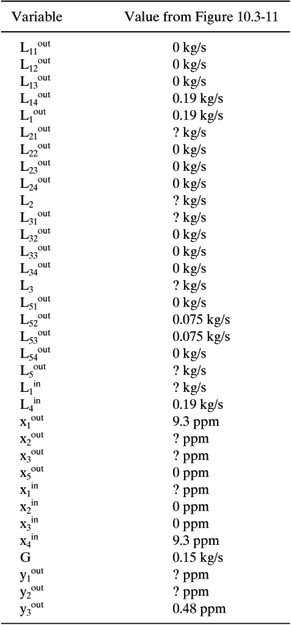
Figure 10.3-11 Diagram of original chloroethane process in the format of Figure 10.3-10.
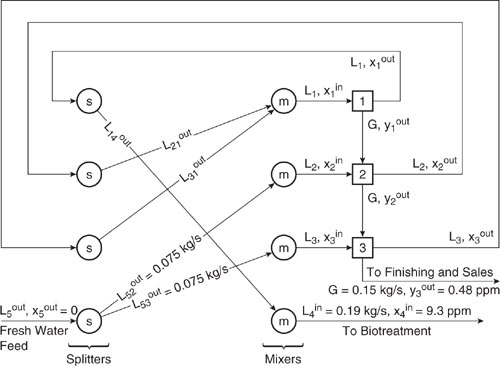
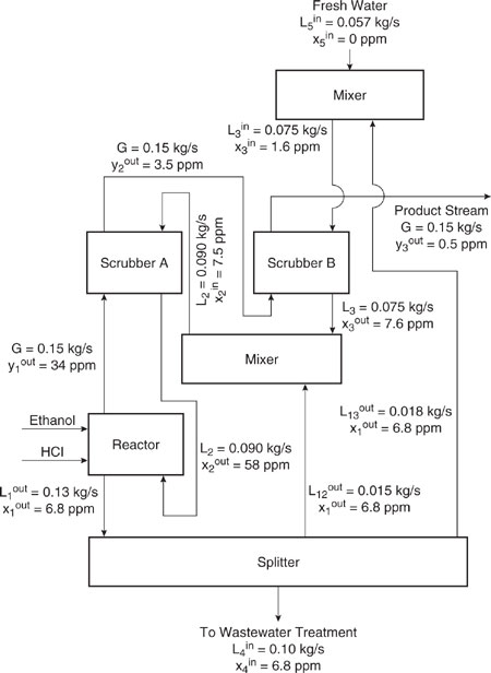
The optimal mixing and recycle rates, where optimal is defined as the process that generates the least amount of chloroethanol, can be determined using linear programming methods. The details are described by El-Halwagi (1997). The original process is shown in Figure 10.3-11 and the optimized process is shown in Figure 10.3-12 and Table 10.3-4.
Table 10.3-4 compares chloroethanol generation, wastewater flow rates, chloroethanol load to the wastewater treatment unit, and fresh water input between the optimized and the original process. Fresh water usage in the proposed process is 38% of that in the original process, and the load to the wastewater treatment unit is decreased from 0.19 kg/s to 0.10 kg/s. Chloroethanol loading to the wastewater treatment unit is decreased from 1.8 mg/s to 0.68 mg/s. Finally, the rate of generation of chloroethanol in the reactor is reduced from 1.9 mg/s to 0.76 mg/s.
Table 10.3-4 Chloroethane Process Characteristics Before and After Optimizing the Segregation, Mixing, and Recycle Strategy.
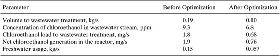
Figure 10.3-12 Chloroethane process with mixing, segregation, and recycle strategy that minimizes the production of chloroethanol.
10.3.3 Mass Exchange Network Synthesis
One of the more rigorous flowsheeting tools for mass integration is mass exchange network (MEN) synthesis. MEN synthesis is analogous to heat exchange network (HEN) synthesis, which was discussed earlier in this chapter. However, while the goal of HEN synthesis is energy efficiency, the goal of MEN synthesis is mass efficiency.
Unlike source-sink mapping and optimizing segregation, mixing, and recycle, MENs do not achieve mass integration through re-routing of process streams. Instead, they involve direct exchange of mass between streams. MEN synthesis was originally developed by Manousiouthakis and coworkers at UCLA (see, for example, El-Halwagi and Manousiouthakis, 1989), and is used to systematically generate a network of mass exchangers whose purpose is to preferentially transfer compounds that are pollutants in the streams in which they are found to streams in which they have a positive value. MEN synthesis can be used for any countercur-rent, direct-contact mass-transfer operation, such as absorption, desorption, or leaching.
The case of phenol at petroleum refineries provides an example of a potential use of an MEN for pollution prevention. In these refineries, phenol is a pollutant in the water effluent of catalytic cracking units, desalter wash water, and spent sweetening waters. In other refinery streams, however, phenol can be a valuable additive. An MEN might therefore be used to transfer phenol to the streams where its presence is desirable, thus preventing phenol pollution in refinery wastewaters.
Remember from the earlier section in this chapter on heat integration that the limits to heat transfer are determined by energy balances and a positive driving force. Similarly, mass transfer is limited by mass balance constraints and equilibrium constraints. The constraints are (1) the total mass transferred by the rich stream (the stream from which a material is to be removed) must be equal to that received by the lean stream (the stream receiving the material) and (2) mass transfer is possible only if a positive driving force exists for all rich stream/lean stream matches. The means of incorporating the constraints into MEN synthesis are discussed in more detail below.
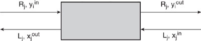
Because it has a positive value in some streams and cannot be referred to as a pollutant, the compound whose transfer is desired will be identified as the “solute” in the discussion that follows. A mass balance on the solute to be transferred from stream i to stream j of Figure 10.3-13 results in the equation
![]()
where Ri is the flow rate of rich stream i, Lj is the flow rate of lean stream j, y i is the mass fraction of the solute in rich stream i, and x j is the mass fraction of the solute in lean stream j. Note that rich streams are streams in which the solute concentration is higher than desired, and lean streams are streams in which the concentration of the solute is lower than desired. For the analysis in this chapter, the flow rates of the streams are assumed to be constant. This is a good approximation if the concentration of solute in the streams is low and little transfer of material other than solute occurs.
Figure 10.3-13 Mass balance diagram for mass exchange network synthesis
Equilibrium between a rich and a lean stream can be represented by an equation of the form
![]()
where xj* is the mass fraction of the solute in stream j that is in equilibrium with the mass fraction yi in stream i and m and b are constants. This linear type of equilibrium relationship is found in familiar expressions such as Raoult’s Law, Henry’s Law, and octanol/water partition coefficients. The constants of Equation 10-24 are thermodynamic properties and may be obtained through experimental data. The positive driving force constraint for mass transfer is satisfied when xj is larger than xj*.
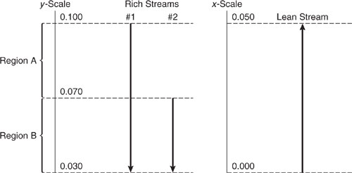
The tools of MEN synthesis are composition interval diagrams and load lines. A composition interval diagram (CID) depicts the lean and rich streams that are under consideration. CIDs for the rich and lean streams of Table 10.3-5 are shown in Figure 10.3-14. To construct this diagram, an arrow is drawn for each stream with its tail at the entering mass fraction and its head at the exiting mass fraction. The following example provides further illustration of the process of mapping lean and rich streams onto a CID.
Table 10.3-5 Stream Data for Two Rich Streams and One Lean Stream.
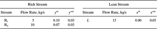
Figure 10.3-14 Composition interval diagram for the streams of Table 10.3-5.
Example 10.3-3 Constructing a Composition Interval Diagram
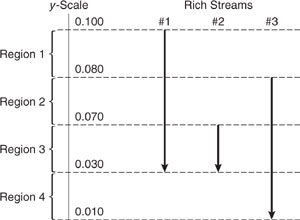
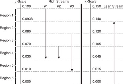
Construct a CID for the rich streams of Table 10.3-6. With the aid of this CID, calculate the mass transferred out of the rich streams in units of kg/s within each region of the CID. The mass transferred from the rich streams within each region is equal to (yout-yin)* _Ri, where yout and yin are the exiting and entering rich stream mass fractions, respectively, and _Ri is the sum of the rich stream flow rates in the region. Note that mass transfer is negative for the rich streams because they are losing mass.
Solution: The rich streams are mapped from Table 10.3-6 to generate the CID shown in Figure 10.3-15. The mass transferred in each region is:
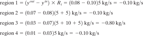
Table 10.3-6 Stream Data for Three Rich Streams and One Lean Stream.

Figure 10.3-15 Composition interval diagram for the rich streams of Table 10.3-6 for Example 10.3-3.
In Figure 10.3-14, the compositions of the rich and lean streams are on sepa-rate axes. These axes can be combined by applying the equilibrium relationship. If the equilibrium relationship in the region of interest for the species considered in this problem is given by
y=0.67x*,
then a mass fraction of y=0.1 in the rich stream is in equilibrium with a mass fraction of x*=0.15 in the lean stream. By converting the lean stream compositions of Figure 10.3-14 to the rich stream compositions with which they are in equilibrium, and vice versa, a combined CID with shared axes as shown in Figure 10.3-16 can be constructed.
Figure 10.3-16 Combined composition interval diagram for the streams of Table 10.3-5.
Example 10.3-4 Constructing a Combined Composition Interval Diagram
Construct a CID for the three rich streams and the lean stream of Table 10.3-6. The equilibrium relationship in the region of interest is
y=0.67x*.
Solution: The combined CID is pictured inFigure 10.3-17.
Figure 10.3-17 Combined composition interval diagram for the streams of Table 10.3-6 for Example 10.3-4.
Load lines depict the flow rate of solute transferred as a function of stream composition. These load lines are drawn on a set of axes that parallel the axes used for HEN synthesis (see Figure 10.2-3. The difference is that instead of heat transfer on the y-axis, mass transfer is used, and instead of temperature on the x-axis, concentration of the solute is used.
Constructing load lines for single streams is best explained through an example. Take R1 of Table 10.3-5. At its inlet, this stream has not begun exchange of solute, so one endpoint of its load line is yin=0.10, mass exchanged 0 kg/s. At its outlet, this stream has exchanged 5 kg/sx (0.03 - 0.10) or - 0.35 kg/s, so the coordinates of the other endpoint are (0.03, - 0.35 kg/s). The amount of mass transferred is negative at this endpoint because mass is being transferred out of the stream. This load line is shown in Figure 10.3-18. Note that there is an arrow pointing down and to the left to indicate the direction of transfer. In the following example, you are asked to construct the load line for the remaining stream of Table 10.3-5.
Figure 10.3-19 Load line for rich stream 1 of Table 10.3-5

Example 10.3-5 Constructing Load Lines
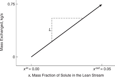
On separate sets of axes, construct load lines for R2 and L of Table 10.3-5. Remember that mass exchanged is equal to the flow rate multiplied by mass fraction out less mass fraction in.
Solution: One end point of the rich stream is at y2in, where no mass has been exchanged. Therefore, at kg/s = 0, y = 0.07. The other end point is (0.03,10 kg/s x (0.03 - 0.07) = -0.4 kg/s). The end points of the lean stream load line are 0 kg/s, x = 0 and 0.75 kg/s, x = 0.05. Plotting these points on the given axes, the graphic relationship between mass transferred (kg/s) and mass fraction shown in Figures 10.3-19 and 10.3-20is obtained. Note that the slope of the load line for the rich stream is (0.4-0)/(0.07 0.03) or 10 kg/s, which is the same as its flow rate. The same is true of the lean stream load line.
Figure 10.3-19 Load line for rich stream 2 of table 10.3-5 for Example 10.3-5.
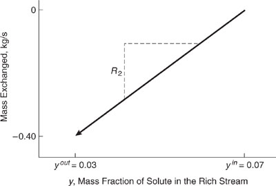
Figure 10.3-20 Load line for the lean stream of Table 10.3-5 for Example 10.3-5.
The load lines of Example 10.3-5 are for a single rich and a single lean stream. When there is more than one rich stream or more than one lean stream to consider, a line representative of the multiple streams must be constructed. This line, called a composite load line, is the sum of the individual load lines and is developed with the aid of a CID.
As an illustration, the composite load line for the rich streams of Table 10.3-5 is plotted in Figure 10.3-21. This composite line is the sum of the load lines of Figures 10.3-18 and 10.3-14. It consists of two segments, corresponding to the regions shown in the CID of Figure 10.19. In region A are the rich streams with mass fractions less than 0.1 and greater than 0.07 (0.1≤y≤0.07). Only R1 falls into this category, so the total flow rate of the rich streams in this composition range is 5 kg/s. The starting point for the load line is y 0.1 and 0.0 kg/s transferred. Re-call that the mass transferred in each CID region is equal to the mass fraction exiting the region minus the mass fraction entering the region, multiplied by the sum of the flow rates in the region. Therefore, at y 0.07, 5 kg/s (0.07 0.1) or 0.15 kg/s have been transferred, and the end point of the load line in this region is (0.07, 0.15 kg/s). As before, the slope of the load line equals the mass flow rate of the stream. In region B are the rich streams with mole fractions less than 0.07 and greater than 0.03. Both rich streams fall into this region, and the endpoint of this
Figure 10.3-21 Composite load line for the rich streams of Table 10.3-5.

segment of the load line is y = 0.03, mass transferred = -0.15 kg/s+ 15 kg/sx(0.03 - 0.07) = - 0.75 kg/s. When the load line is plotted, it has a slope equal to the sum of the flow rates of all streams in this region. The starting point for this segment of the load line is the termination point of the previous segment.
Example 10.3-6 Constructing a Composite Load Line
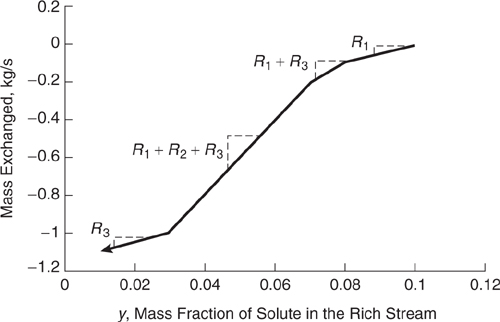
Plot the composite load line for the rich streams of Table 10.3-6. Based on the total amount of mass transferred from the rich streams, calculate the minimum flow rate required for the lean stream. In the example that follows, the validity of using this simple overall mass balance technique for determining the minimum lean stream flow rate is examined.
Solution: The end points for the segments of the composite load line for the rich streams are: (0.1,0),(0.08,- 0.10 kg/s), (0.07,- 0.20 kg/s), (0.03,- 1.0) and (0.01,- 1.1). See Figure 10.3-22. Note that to plot a continuous load line, the cumulative mass transferred is used; the mass transferred in each interval is added to the mass transferred in all previous intervals. If the mass transferred by rich streams equals the mass gained by the lean stream, and (from before) total mass transferred from the rich streams is 1.10 kg/s, then from Table 10.3-6, mass gained by the lean stream is equal to L(0.14- 0.0), where L is the flow rate of the lean stream. Thus,
L(0.14 - 0.0) = 1.10
or
L= 7.86 kg>s.
Figure 10.3-22 Composite load line for the rich streams of Table 10.3-6 for Example 10.3-6.
The next step in constructing load line diagrams is to plot the lean and rich streams on the same axes. As with combined CIDs, load line diagrams can be combined by making use of the equilibrium relationship, which for this specific numerical example is assumed to be
y=0.67x*
in the region of interest.
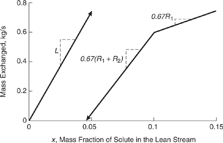
A combined figure can be made by following several different conventions, each of which gives the same final results. The convention used here for constructing the combined figure for the streams of Table 10.3-5 is to first plot the load line of the lean stream as shown in Figure 10.3-23. The rich stream composite load line is added to the figure after converting the rich stream mass fractions into the lean stream mass fractions with which they are in equilibrium. These conversions were made in order to construct the CID of Figure 10.3-16. The rich stream composite load line is free to move vertically; its placement determines which lean and rich streams contact each other. The rich stream load line has this freedom to move vertically because the values for mass exchanged on the y-axis are not absolute: they are useful only in relative terms, i.e., in terms of the differences in mass transferred between points. Therefore, the composite rich stream load line begins at x* (the x-axis) = lean stream mass fraction with which the rich stream is in equilibrium = 0.10/0.67 = 0.15 and continues downward and to the left with a slope of 0.67R1. The next point falls at x = 0.07/0.67 = 0.10 where the slope changes to 0.67(R1 + R 2). The load line ends where x = 0.03/0.67 = 0.045. The load lines for the lean and rich streams of Table 10.3-5 are plotted together in Figure 10.3-23. As stated before, the composite rich stream load line could have been located in any number of different vertical positions.
Figure 10.3-23 Combined load line diagram for the streams of Table 10.3-5.
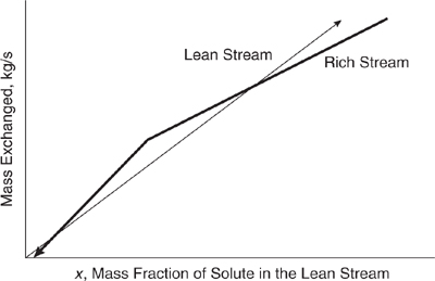
In Figure 10.3-23, the lean stream load line falls to the left of the composite rich stream load line at every point. This indicates that the desired mass exchange is thermodynamically feasible (i.e., the equilibrium constraint is satisfied), and that the transfer could be accomplished using exchangers of finite size with no need for mass exchange into or out of any other streams. In Figure 10.3-24, the lean stream load line lies to the left of the rich stream load line, except at a point, called the pinch point, where the lines meet. Mass exchange in a case such as this is thermo-dynamically feasible, but would require an infinitely large mass exchanger (an infinite number of trays or stages, for example). Therefore, there is a practical requirement that conditions be manipulated so that a positive horizontal ? exists between the load lines. This ? is the driving force for mass transfer. If at any point the lean stream load line lies to the right of the rich stream load line, as shown in Figure 10.3-25, mass exchange in the desired direction is not thermodynamically feasible. In fact, if streams with such characteristics are contacted, mass exchange from the lean stream to the rich stream occurs. This infeasible situation could be made feasible by moving the rich stream load line down.
Figure 10.3-24 Load lines form a pinch.
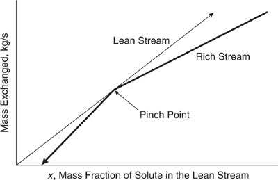
Figure 10.3-25 Mass transfer is thermodynamically infeasible where the rich stream load line lies to the left of the lean stream load line.
Example 10.3-7 Plotting Rich and Lean Stream Load Lines on a Single Set of Axes
Using the CID generated in Example 10.3-5, plot the load lines of the rich and lean streams described in Table 10.3-6 on the same diagram so that a pinch exists. Assign the lean stream a flow rate of 8 kg/s. Can the specified target concentrations be achieved solely through contact between the lean and rich streams? What does this indicate about the solution in Example 10.3-6 for the minimum lean stream flow rate required? Is there a lean stream flow rate at which all the desired mass exchange can occur solely through contact between the streams? If yes, what is that flow rate?
Solution: The easiest way to add the composite rich stream load line to the lean stream diagram is to determine where the pinch point occurs, plot it, and work outward. From examination of Figure 10.3-22, it appears that the point where x = 0.07/0.67 = 0.104 is the pinch point. The value for mass exchanged at this point is found using the equation for the lean stream load line, which is
mass exchanged = (8kg/s)x.
Therefore, the first point to plot for the composite rich stream load line is(0.104, 8(0.104)kg/s = 0.832 kg/s). See Figure 10.3-26 for the remaining points on the composite rich stream load line. Target concentrations cannot be achieved solely through contact between the streams because the target concentration of the rich stream is lower than its concentration after contact with the lean stream (bottom left of Figure 10.3-26) and because the target concentration of the lean stream is higher than its concentration after contact with the rich stream (top right of Figure 10.3-26).
Figure 10.3-26 Combined load line diagram for the streams of Table 10.3-6 for Example 10.3-7
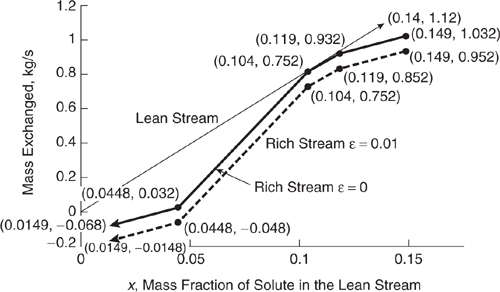
The lean stream flow rate here (8 kg/s) is greater than the minimum lean stream flow rate calculated in Example 10.3-6, but it is insufficient to effect all the necessary mass exchange. There is no lean stream flow rate at which all the desired mass exchange can be achieved solely through contact between the streams.
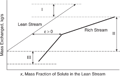
Diagrams that combine the rich and lean stream load lines also show the amount of excess mass transfer capacity available from the lean stream and the amount of excess mass transfer capacity available from the rich stream. These regions were deliberately, if unrealistically, omitted in Figures 10.3-23, 10.3-24, and 10.3-25 for the sake of illustrating thermodynamic feasibility. In Figure 10.3-27, three regions labeled I, II, and III are identified. In region I, the lean stream has the capacity to exchange more mass and become richer, but there is a “shortage” of rich stream. The lean stream must be brought up to its specified concentration in a manner other than through mass exchange with the rich stream. For instance, the solute may be added to it. In region II, mass exchange can occur through contact between the rich and lean streams. In region III, the rich stream is capable of mass exchange, but there is a “shortage” of lean stream. An external lean stream mass separating agent is required to achieve the rich stream’s target concentration. For example, an adsorbent such as activated carbon might be used to take up the excess solute, which is a pollutant in the rich stream. For the lean and rich streams depicted in Figure 10.3-27, the least amount of solute and external lean stream or mass separating agent is required when the rich stream load line is manipulated to form a pinch point (ε = 0). As ε increases, operating costs (the cost of solute and the cost of the mass separating agent) increase and capital costs (the cost of the network) decrease. As ε decreases, operating costs decrease and capital costs increase.As with HEN synthesis, it is possible to find the ε at which total annualized costs are minimized.
Figure 10.3-27 The three regions of a combined load line diagram.
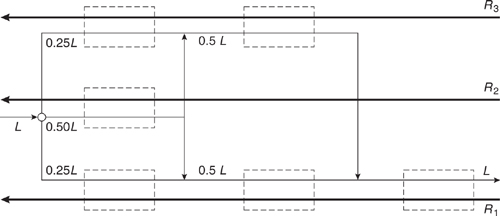
MEN synthesis is powerful because of its graphic determination of the pinch point and its ability to show whether mass exchange is thermodynamically feasible. The culmination of all the previous steps is the synthesis of a mass exchange network. Combined load line diagrams show where the lean and rich streams contact each other in a mass exchange network. For example, inspection of Figure 10.3-26 reveals that rich stream 1 contacts the lean stream as the lean stream exits the mass exchange network. Then, where the lean stream mass fraction is 0.60/L1 = 0.04, the lean stream is split and one third contacts rich stream 1 while the remaining two thirds contacts rich stream 2. The lean stream enters this mass exchange network at the same point where both rich streams exit.
Example 10.3-8 Pairing Streams in a Mass Exchange Network (adapted from Allen and Rosselot, Pollution Prevention for Chemical Processes © 1997. This material is used by permission of John Wiley & Sons, Inc.)
Describe how the streams contact each other in the optimal mass exchange network of Figure 10.3-26. (This is the network where the value of _ is equal to 0.01.) To begin, rich stream 1 contacts the lean stream when the lean stream exits the mass exchange network. Further down the mass exchange network, the lean stream is split into two parts, with one third contacting rich stream 1 and two thirds contacting rich stream 2. Complete this description for the mass exchange network, and give the lean stream and rich stream mass fractions at which the splits/junctions occur.
Solution: As stated in the problem statement, rich stream 1 contacts the lean stream where the lean stream exits the mass exchange network. At this point, the mass fraction of solute in the lean stream is 0.952 kg/s/8kg/s = 0.119 (found from the equation of the lean stream load line) and the rich stream mass fraction is 0.149 × 0.67 = 0.10 (read directly from the composition interval diagram). Where the lean stream mass fraction is 0.852/8 = 0.107 and the rich stream mass fraction is 0.119 × 0.67 = 0.08, the lean stream is split, with one half contacting rich stream 1 and the other half contacting rich stream 3. The lean stream is split three ways when its mass fraction is 0.752/8 = 0.094 and the rich stream mass fraction is 0.104 × 0.67 = 0.07, with one fourth contacting rich stream 1, one half contacting rich stream 2, and the remaining fourth contacting rich stream 3. To find the mass fraction of solute in the lean stream when the rich streams exit the mass exchange network, the equation of the corresponding portion of the composite rich stream load line must first be found. It is known that the slope of this line is
m = 0.67(R1 + R2 + R3) = 13.4kg/s.
The intercept is found by using one of the known points as follows:
0.752 kg/s = 13.4kg/s(.07/.67) + b.
Therefore, b = —0.648 kg/s. The mass fraction at which this line crosses the x-axis can be found from
0 = (13.4 kg/s)x — 0.648 kg/s.
This means that the rich streams exit the mass exchange network when the mass fraction of solute in them is 0.67 × 0.648/13.4 = 0.0324. The lean stream mass fraction at this point is 0. See Figure 10.3-28 for a flowsheet of this network. Stream matching around the pinch point is particularly complex (see Douglas, 1988 and El-Halwagi, 1997). MEN synthesis is described in more detail in El-Halwagi, 1997.
Figure 10.3-28 Mass exchange network showing stream matching for the streams of Table 10.3-6. Dashed lines indicate mass exchange units for Ex10-3-8 Example 10.3-8.
Case Study of a Process Flowsheet
In this section, the process flowsheet for a generic crude oil processing unit at a petroleum refinery is described, along with pollution prevention techniques that were developed for the unit (American Petroleum Institute, 1993). These pollution prevention techniques demonstrate the usefulness of both qualitative and quantitative flowsheeting tools and illustrate the complexity and integration found in processes in the chemical processing and refining industries. In this case study, proposed pollution prevention techniques, including both heat and mass integration, result in substantial environmental improvements at a cost savings.
One of the largest processing units in a petroleum refinery is the facility that separates crude oil into volatility fractions suitable for further processing (the crude unit). The hypothetical crude unit of this case study processes 175,000 barrels of light Arabian crude oil a day. It consists of a desalter (which removes salt and other contaminants from crude oil), an atmospheric distillation tower (so-called because it operates at atmospheric pressure), and a vacuum distillation column (which operates at lower-than-atmospheric pressure in order to allow the column to separate low volatility materials at acceptable temperatures), as shown in Figure 10.4-1. Crude oil and water are the primary feed materials and several output streams are produced, including crude tower overhead (fuel gas and unstabilized gasoline), a light naphtha fraction, a kerosine fraction, a heavy distillate fuel fraction, an atmospheric gas oil (heavy) fraction, light vacuum gas oil, heavy vacuum gas oil, and vacuum residue.
While the crude unit is one of the largest processing units at a petroleum refinery, it is important to remember that at a typical refinery, the streams from the crude unit are sent to many other processing units, many of which are reactors whose purpose is convert large hydrocarbon molecules into more saleable products. These reactors include fluidized-bed catalytic crackers, hydroprocessers, and cokers. Other reactors create compounds with a higher octane rating, or combine small hydrocarbon compounds to create larger ones. Still other downstream processing units are used to purify and blend the refinery process streams. Finished refinery products include gasoline, jet fuel, diesel fuel, fuel oil, waxes, asphalt, and petrochemical feedstocks. The boundaries of this case study, however, include only the crude unit and its input and output streams. The first major process unit, shown in Figure 10.4-2, is the desalter. Desalting removes salts in the crude that would cause corrosion of the process equipment. It also removes metals and suspended solids that would foul catalysts in downstream processing units.
In the first step of the desalting process, the crude oil is mixed with partially treated wastewater recycled from the refinery. Next, the oil is heated using a series of heat exchangers in preparation for desalting. In the desalter, which has two stages, hot oil and hot recycled water create a dispersed mixture of oil and water. The water extracts additional salts from the oil, and the salt-rich water (brine) is separated from the oil using an electric field. The brine from the desalter’s second stage is used as the wash water for the first stage, and brine from the first stage is sent to wastewater treatment after being cooled by heat exchange with desalter feed water and cooling water. The desalted crude is then sent to another series of heat exchangers, which elevate its temperature to 424°F.
Figure 10.4-1 A simplified schematic of the petroleum refining cude unit.

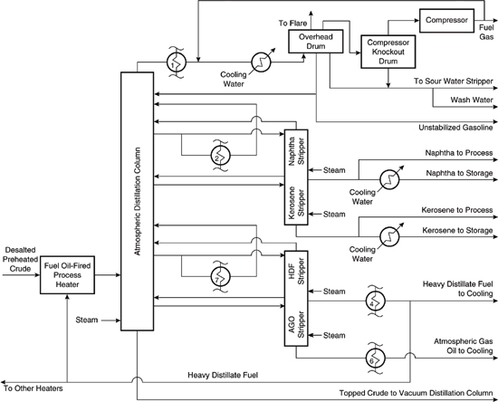
After desalting and preheating, the crude oil is sent to the atmospheric pressure distillation process unit, shown in Figure 10.4-3. Fuel-fired heaters supply energy to the tower. Note that several streams are withdrawn from the column. Two of the side streams removed from the tower are sent to secondary strippers, where they are contacted with steam, and the products from these separation operations are sent to further processing operations at the refinery. The overhead product from the atmospheric distillation tower is cooled by heat exchange with the incoming crude oil and with cooling water. This overhead stream is collected in a drum and the fuel gases in the vapor phase are withdrawn, compressed, and sent to further processing operations at the refinery. Part of the gasoline in the condensed phase is used as a reflux for the atmospheric pressure distillation tower and the remainder is sent to the refinery. The bottom stream from the distillation column is sent to the next major process unit, the vacuum distillation tower.
Figure 10.4-2 The desalter and crude oil preheaters for the hypothetical petroleum refining crude unit. Heat exchangers are numbered for cross-reference with Figures 10.4-3 and 10.4-4.

Figure 10.4-3 The atmospheric distillation tower for the hypothetical petroleum refining crude unit. Heat exchangers are numbered for cross-reference with Figure 10.4-2.
In the vacuum distillation unit, shown in Figure 10.4-4, the bottoms from the atmospheric distillation unit are further fractionated into vacuum tower overhead, light vacuum gas oil, heavy vacuum gas oil, and vacuum tower bottoms. The energy for the tower is provided by a fuel-fired heater. Most of the product streams are sent directly to downstream processing at the refinery, with the exception of the overhead stream. The overhead stream is contacted with steam, then cooled and sent to a collection vessel called the overhead drum, where the oil and water phases are sepa-rated. The water stream from the overhead drum (which is contaminated with ammonia, hydrogen sulfide, and other components) is sent to the refinery’s sour water stripper, which is a wastewater treatment process that recovers ammonia and hydrogen sulfide. The oil recovered from the overhead drum is sent to storage.
It is clear from this simplified process description that the crude unit in a refinery is a complex process that generates a variety of gaseous, liquid, and solid wastes. These wastes and emissions are described in Table 10.4-10.
Qualitative techniques for identifying pollution prevention opportunities were used to develop most of the proposed pollution prevention options for the crude unit. These options are described below:
1. Reboil with hot oil rather than steam to avoid oil/water contacting operations. Two additional side strippers must be added to the tower when this is done because the product specifications cannot be met with the existing side strippers when hot oil is used instead of steam for reboiling.
2. Add a liquid ring vacuum pump to the vacuum tower in order to reduce the pressure in the vacuum tower, which results in lower allowable operating temperatures, which in turn results in reduced cracking and fouling of the furnace tubes in the furnace, so that production of sour water is reduced.
3. Replace burners with new generation low-NOx burners and retrofit for flue-gas recirculation in order to reduce NOx emissions.
4. Reduce fugitive emissions by implementing a stringent inspection and maintenance program for piping components, using leakless valves when replacing small valves wherever it is economical to do so, using graphite or teflon packing and seals when repairing valves, specifying double seals when replacing pumps, installing rupture disks on pressure relief valves and venting them to a flare, modifying the compressor, blind-flanging all the vents and drains, eliminating flanges where possible, and making all the sampling systems closed-loop.
5. Segregate mildly-contaminated wastewater and treat it so that it can be reused.
In addition to the above strategies, pinch analysis to reduce external energy requirements showed that air emissions could be reduced substantially by increasing the surface area of the existing preheaters by 8% by adding three additional pre-heaters. The capital cost of these preheaters was estimated to be $2,268,000, while the annual savings in fuel costs were estimated to be $1,692,000. Therefore, the additional heat exchangers were projected to have a payback period of one and a third years.
Figure 10.4-4 The vacuum distillation tower for the hypothetical petroleum refining crude unit. Heat exchangers are numbered for cross-reference with Figure 10.4-2.

Table 10.4-1 Major Waste and Emission Streams from a Petroleum Refining Crude Unit.

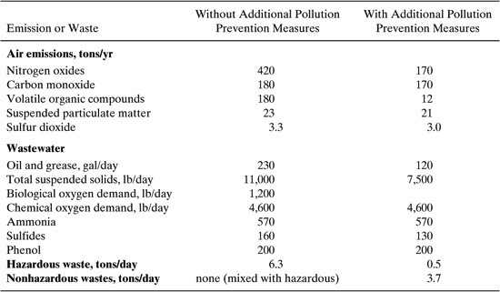
Table 10.4-2 shows estimated wastes and emissions for the hypothetical crude processing unit with and without the pollution prevention measures. The measures were projected to decrease emissions of nitrogen oxides to air by 60%, and volatile organic compound emissions to air were projected to decrease by 93%. The quantity of oil and grease in wastewater was nearly halved, total suspended solids in wastewater were decreased by 32%, and sulfides in wastewater were decreased by 19%. Production of hazardous solid waste was decreased by over 90%, and a nonhazardous waste stream was generated.
Table 10.4-2 Estimates of Crude Unit Emissions and Waste Generation Before and After Pollution Prevention Alternatives are Implemented.
Summary
Even the simplest of chemical processes generally consist of a number of process units whose characteristics can influence overall waste generation. In this chapter, it was shown that pollution prevention can sometimes be achieved by examining the mass and energy integration of process units. Qualitative and quantitative tools for analyzing flowsheets are described. Case studies, in both the text of the chapter and in the accompanying problems, reveal both the power and the complexity of process integration.
References
Allen, D.T. and Rosselot, K.S., Pollution Prevention for Chemical Processes, Wiley-Interscience, New York, 1997.
American Petroleum Institute (API), Environmental Design Considerations for Petroleum Refining Crude Processing Units, Publication 311, Washington, DC, 1993.
Crowl, D. A. and Louvar, J. F., Chemical Process Safety: Fundamentals with Applications, Prentice-Hall, Englewood Cliffs, NJ, 1990.
DuPont (1993), “DuPont Chambers Works Waste Minimization Project: Cambers Works— Deepwater, New Jersey,” Report to the U.S. Government in satisfaction of consent decree in U.S.v. DuPont, Docket No.91cv768(JFG), May, 1993.
Douglas, J.M., Conceptual Design of Chemical Processes, McGraw-Hill, New York, 1988.
Douglas, J.M., “Process Synthesis for Waste Minimization,”Industrial and Engineering Chemistry Research,31, 238-243, 1992.
El-Halwagi, M. and Manousiouthakis, V., “Synthesis of Mass Exchange Networks”, AIChE Journal, 35, 1233-1244 (1989).
El-Halwagi, M., Pollution Prevention Through Process Integration: Systematic Design Tools, Academic Press, San Diego, CA, 1997.
Rossiter, A. P. and Klee, H., “Hierarchical Process Review for Waste Minimization,” Waste Minimization Through Process Design, A. P. Rossiter, ed., McGraw-Hill, New York, 1995.
Problems
1. Determine the amount of energy savings that could be achieved by putting in place a heat exchange network in the hot water system for a typical house.
a) Begin by identifying the hot water streams from which heat can be extracted (e.g., dishwasher effluent, shower effluent). For each of these streams, estimate a water exit temperature and a daily flow rate.
b) Assume that these hot streams will be contacted with the cold supply water entering the hot water heater and estimate the amount of energy that could be extracted from the hot streams. Determine the annual energy savings if the home uses an electric hot water heater and electricity costs $0.06/kwh. Make reasonable assumptions about the efficiency of the hot water heater (fraction of the electricity that goes into heated water used by the homeowner).
c) The cost of an installed, non-contact, single tube, shell and tube exchanger for this application is approximately $500. Assume that the hot water exit lines al-ready pass near the water heater so that little additional plumbing is required. Determine the time required to repay the installation cost using money saved in energy costs.
2. The equilibrium between the rich stream and the lean stream listed below is:
y = 1.5 x 0.8
Rich stream 1: yin = 0.45 yout = 0.1 Flowrate = 3 kg/s
Lean stream: xin = 0.45 xout = 0.1 Flowrate = 5 kg/s
A second rich stream is available. The equilibrium relationship between the second rich stream and the lean stream is:
y = 1.5x
The second rich stream has inlet and outlet concentrations listed below.
Rich stream 2: yin = 0.3 yout = 0.1 Flowrate = 3kg/s
3.Recovery of Benzene from the Aqueous Wastes of a Styrene Manufacturing Process (adapted from El-Halwagi, 1997). Styrene is manufactured by dehydrogenating ethylbenzene over an oxide catalyst at 600 to 650°C. Steam is generally co-injected with the ethylbenzene into the reactor, shown in Problem 3, Figure 1. Styrene and hydrogen gas are the primary reaction products. Byproducts include benzene, ethane, toluene and methane. The products and byproducts from the reactor are cooled to approximately ambient temperature. Light products such as hydrogen, methane and ethane which do not condense when cooled to ambient temperatures are vented. The condensed materials are sent to a decanter where an organic layer and an aqueous layer form. The organic layer containing benzene, toluene, and unreacted ethyl-benzene is recycled. The aqueous portion of the wastewater stream (R2) generated in the decanter is saturated with benzene and must be treated.
Problem3, Figure1. Flow diagram for styrene manufacturing facility
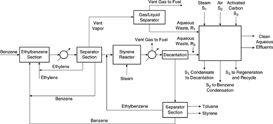
Another wastewater stream (R1) is generated earlier in the process, during the manufacture of ethylbenzene. The ethylbenzene fed to the styrene manufacturing operation is generally produced on site from ethylene and benzene and produces a condensate wastewater stream that is saturated with benzene.
Thus, there are two sources of benzene saturated wastewater (approximately 1770 ppm or 0.00177 kg benzene/kg water) in the process: R1 (1000 kg/hr) and R 2(69,500 kg/hr). The concentrations of benzene must be reduced to at most 57 parts per billion in the wastewater.
Design a recycle and reuse system for the benzene using steam stripping and adsorption onto activated carbon. The system is shown in Problem 3, Figure 2. In the design:
• A steam stripping unit is used which removes benzene from the wastewater and recycles it. This unit produces a wastewater stream saturated with benzene (70 kg/h; see Problem 3, Figure 2) that must be sent to the recovery system.
• Spent activated carbon is regenerated with steam. The steam is recovered by condensation, producing a wastewater stream saturated with benzene (37 kg/h; see Problem 3, Figure 2). This wastewater is sent to the benzene recovery system.
a) Draw a composition interval diagram for the benzene rich streams.
b) Data on the lean stream compositions are given below. The target compositions are based on a variety of factors. For example, the supply composition of benzene in activated carbon corresponds to the residual benzene remaining on the carbon after regeneration. Using these data, draw the composition interval diagram for the lean streams.

c) Using the equilibrium relationships shown below, draw a pinch diagram for this system.
yi = mi × xi
where yi and xi are the mass ratios (kg benzene/kg benzene free stream) in the rich and lean streams. Assume mi for steam is 0.001 and mi for activated carbon is 0.00071.
d) Determine the location of the pinch point assuming no minimum driving force for mass transfer and calculate the amount of benzene recovered. What is the value of the recovered benzene if it can be sold for $0.20/kg? Repeat your calculation for a minimum mass transfer driving force of 0.001.
e) Compare your results to the flow rates shown in Problem 3, Figure 2 and discuss any differences.
Problem3, Figure2. Mass exchange network for the styrene facility. All flow rates are in kg of benzene free stream per hour; numbers without units represent mass ratios, in kg of benzene per kg of benzene free stream.

4. Etching of copper, using an ammoniacal solution, is an important operation in the manufacture of printed circuit boards. During etching, the concentration of copper in the ammoniacal solution increases. Etching is most efficiently carried out for copper concentrations between 10 and 13 weight% in the solution, while etching efficiency almost vanishes at higher concentrations (15–17 weight%). In order to maintain the etching efficiency, copper must be continuously removed from the spent ammoniacal solution through solvent extraction. The regenerated ammoniacal etchant can then be recycled to the etching line.
The etched printed circuit boards are washed with water to dilute the concentration of the contaminants on the board surface to an acceptable level. The extraction of copper from the effluent rinse water is essential for both environmental and economic reasons, since decontaminated water is returned to the rinse vessel.
A flowsheet of the etching process is shown in Problem 4, Figure 1.
Design a mass exchange network that will recover copper from the rinse water and spent ammoniacal etchant. The characteristics of the rich streams are:

Problem4, Figure1 Flowsheet for copper etching process described in Problem 4.

Two lean streams are available. One lean stream for extracting copper is an aliphatic hydroxyoxime (S1). It can be loaded to a copper mass fraction of 0.07. When regenerated, it has a copper mass fraction of 0.03. The equilibrium relationship between this lean stream and the two rich streams is given by:
y = 0.734x + 0.001
where y is the rich stream copper mass fraction and x is the lean stream copper mass fraction.
A second lean stream for extracting copper is an aromatic hydroxyomine (S2)It can be loaded to a copper mass fraction of 0.2. When regenerated, it has a copper mass fraction of 0.001. The equilibrium relationship between this lean stream and the two rich streams is given by:
y = 1.5x + 0.1
where y is the rich stream copper mass fraction and x is the lean stream copper mass fraction.
a) Draw a composition interval diagram for the rich streams and the lean streams. Express all concentrations in units of the rich stream mass fractions.
b) Determine the maximum amount of copper that can be removed using S1. What flow rate of S1 does this correspond to?
c) Determine the maximum amount of copper that can be removed using S2. What flow rate of S2 does this correspond to?
d) Determine the maximum amount of copper that can be removed using both S 1 and S2.
e) If the cost of the aromatic stream (S2) is half the cost of the aliphatic stream (S1), identify the optimal ratio of the two lean streams that still recovers the maximum amount of copper.