
Chapter 1
An Introduction to Environmental Issues
1.1 Introduction
Environmental issues gained increasing prominence in the latter half of the 20th century. Global population growth has led to increasing pressure on worldwide natural resources including air and water, arable land, and raw materials, and modern societies have generated an increasing demand for the use of industrial chemicals. The use of these chemicals has resulted in great benefits in raising the standard of living, prolonging human life and improving the environment. But as new chemicals are introduced into the marketplace and existing chemicals continue to be used, the environmental and human health impacts of these chemicals has become a concern. Today, there is a much better understanding of the mechanisms that determine how chemicals are transported and transformed in the environment and what their environmental and human health impacts are, and it is now possible to incorporate environmental objectives into the design of chemical processes and products.
The challenge for future generations of chemical engineers is to develop and master the technical tools and approaches that will integrate environmental objectives into design decisions. The purpose of Chapter 1 is to present a brief introduction to the major environmental problems that are caused by the production and use of chemicals in modern industrial societies. With each environmental problem introduced, the chemicals or classes of chemicals implicated in that problem are identified. Whenever possible, the chemical reactions or other mechanisms responsible for the chemical’s impact are explained. Trends in the production, use, or release of those chemicals are shown. Finally, a brief summary of adverse health effects is presented. This chapter’s intent is to present the broad range of environmental issues which may be encountered by chemical engineers. Chapter 3 contains a review of selected environmental regulations that may affect chemical engineers. It is hoped that this information will elevate the environmental awareness of chemical engineers and will lead to more informed decisions regarding the design, production, and use of chemicals.
1.2 The Role of Chemical Processes and Chemical Products
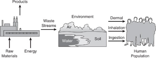
In this text, we cover a number of design methodologies for preventing pollution and reducing risks associated with chemical production. Figure 1.2-1 shows conceptually how chemical processes convert raw materials into useful products with the use of energy. Wastes generated in chemical manufacturing, processing, or use are released to the environment through discharges to streams or rivers, exhausting into the air, or disposal in a landfill. Often, the waste streams are treated prior to discharge.
We may be exposed to waste stream components by three routes: dermal (skin contact), inhalation, and ingestion. The route and magnitude of exposure is influenced by the physical, chemical, and reactivity properties of the waste stream components. In addition, waste components may affect the water quality of streams and rivers, the breathability of ambient air, and the well-being of terrestrial flora and fauna. What information will a chemical engineer need to make informed pollution prevention and risk reduction decisions? A few generalized examples will aid in answering such a question.
Figure 1.2-1 Generalized scenario for exposure by humans to environmental pollutants released from chemical processes.
Formulation of an Industrial Cleaner
Company A plans to formulate a concentrated, industrial cleaner, and needs to incorporate a solvent within the product to meet customer performance criteria. Several solvents are identified that will meet cost and performance specification. Further, Company A knows that the cleaning product (with the solvent) will be discharged to water and is concerned about the aquatic toxicity of the solvent. The company conducts a review of the pertinent data to aid in making the choice. In aquatic environments, a chemical will have low risk potential if it has the following characteristics:
a) High Henry’s Law constant (substance will volatilize into the air rather than stay in the water)
b) High biodegradation rate (it will dissipate before exerting adverse health effects)
c) Low fish toxicity parameter (a high value of the concentration lethal to a majority of test organisms or LC50)
d) Low Bioconcentration Factor, BCF (low tendency for chemicals to partition into the fatty tissue of fish, leading to exposure and adverse health effects upon consumption by humans)
Company A assembles the data and chooses a solvent with the least adverse environmental consequences. Methods are presented in this text to provide estimates of environmental properties. In addition, measured data for some of these properties are tabulated.
Formulation of a Paint Solvent
Company B is formulating a paint for an automobile refinishing. The formulation must contain fast-drying solvents to ensure uniform coating during application. These fast-drying solvents volatilize when the paint is sprayed and are exhausted by a fan. Workers in the booths may be exposed to the solvents during application of the paint and nearby residents may inhale air contaminated by the exhausted solvents.
The company is concerned about the air releases and problems that arise with worker exposure to toxic agents and impact to air quality. A number of solvents having acceptable cost and coating performance characteristics have been identified. A chemical will have low risk potential in the air if it has the following characteristics:
a) Low toxicity properties (high Reference Dose [RfD] for inhalation toxicity to humans or a low cancer potency), and
b) Low reactivity for smog formation (ground level ozone production).
Candidate solvents may be screened for these properties to identify the environmentally optimal candidate.
Choice of Refrigerant for a Low-Temperature Condenser
A chemical engineer is in charge of redesigning a chemical process for expanded capacity. One part of the process involves a vapor stream heat exchanger and a refrigeration cycle. In the redesign, the company decides to use a refrigerant having low potential for stratospheric ozone depletion. In addition, the engineer must also ensure that the refrigerant possesses acceptable performance characteristics such as thermodynamic properties, materials compatibility, and thermal stability. From the list of refrigerants that meet acceptable process performance criteria, the engineer estimates or finds tabulated data for
a) atmospheric reaction-rate constant,
b) global warming potential, and
c) ozone depletion potential.
From an environmental perspective, an ideal refrigerant would have low ozone depletion and global warming potentials while not persisting in the atmosphere.
These three examples illustrate the role the chemical engineer plays by assessing the potential environmental impacts of product and process changes. One important impact the chemical engineer must be aware of is human exposure, which can occur by a number of routes. The magnitude of exposure can be affected by any number of reactive processes occurring in the air, water, and soil compartments in the environment. The severity of the toxic response in humans is determined by the toxicology properties of the emitted chemicals. The chemical engineer must also be aware of the life cycle of a chemical. What if the chemical volatilizes but is an air toxicant? What if the biodegradation products (as, for example, with DDT) are the real concern? For example, terpenes, a class of chemical compounds, were touted as a replacement for chlorinated solvents to avoid stratospheric ozone depletion, but terpenes are highly reactive and volatile and can contribute to photochemical smog formation.
The next sections present a wide range of environmental problems caused by human activities. Trends in the magnitude of these problems are shown in tabular or graphical form, and contributions by industrial sources are mentioned whenever possible. Later chapters develop risk assessment and reduction methods to help answer the questions posed in the previous examples.
1.3 An Overview of Major Environmental Issues
The next several sections present an overview of major environmental issues. These issues are not only of concern to the general public, but are challenging problems for the chemical industry and for chemical engineers. The goal of the following sections is to provide an appreciation of the impacts that human activities can have on the environment. Also, the importance of healthy ecosystems are illustrated as they affect human welfare, the availability of natural resources, and economic sustainability.
When considering the potential impact of any human activity on the environment, it is useful to regard the environment as a system containing interrelated subprocesses. The environment functions as a sink for the wastes released as a result of human activities. The various subsystems of the environment act upon these wastes, generally rendering them less harmful by converting them into chemical forms that can be assimilated into natural systems. It is essential to understand these natural waste conversion processes so that the capacity of these natural systems is not exceeded by the rate of waste generation and release.
The impact of waste releases on the environment can be global, regional, or local in scope. On a global scale, man-made (anthropogenic) greenhouse gases, such as methane and carbon dioxide, are implicated in global warming and climate change. Hydrocarbons released into the air, in combination with nitrogen oxides originating from combustion processes, can lead to air quality degradation over urban areas and extend for hundreds of kilometers. Chemicals disposed of in the soil can leach into undergound water and reach groundwater sources, having their primary impact locally, near to the point of release. The timing of pollution releases and rates of natural environmental degradation can affect the degree of impact that these substances have. For example, the build-up of greenhouse gases has occurred over several decades. Consequently, it will require several decades to reverse or stall the build-up that has already occurred. Other releases, such as those that impact urban air quality, can have their primary impact over a period of hours or days.
The environment is also a source of raw materials, energy, food, clean air, water, and soil for useful human purposes. Maintenance of healthy ecosystems is therefore essential if a sustainable flow of these materials is to continue. Depletion of natural resources due to population pressures and/or unwise resource management threatens the availability of these materials for future use.
The following sections of Chapter 1 provide a short review of environmental issues, including global energy consumption patterns, environmental impacts, ecosystem health, and natural resource utilization. Much of the material presented in this section is derived from the review by Phipps (1996) and from US EPA reports (US EPA, 1997).
1.4 Global Environmental Issues
1.4.1 Global Energy Issues
The availability of adequate energy resources is necessary for most economic activity and makes possible the high standard of living that developed societies enjoy. Although energy resources are widely available, some such as oil and coal are non-renewable, and others, such as solar, although inexhaustible, are not currently cost effective for most applications. An understanding of global energy usage patterns, energy conservation, and the environmental impacts associated with the production and use of energy are therefore very important.
Often, primary energy sources such as fossil fuels must be converted into another form such as heat or electricity. As the Second Law of Thermodynamics dictates, such conversions will be less than 100% efficient. An inefficient user of primary energy is the typical automobile, which converts into motion about 10% of the energy available in crude oil. Some other typical conversion efficiencies are given in Example 1.4-1, below.
Example 1.4-1
Efficiency of Primary and Secondary Energy: Determine the efficiency of primary energy utilization for a pump. Assume the following efficiencies in the energy conversion:
• Crude oil to fuel oil is 90% (.90)
• Fuel oil to electricity is 40% (.40)
• Electricity transmission and distributions is 90% (.90)
• Conversion of electrical energy into mechanical energy of the fluid being pumped is 40% (.40)
Solution: The overall efficiency for the primary energy source is the product of all the individual conversion efficiencies.
Overall Efficiency = (.90)(.40)(.90)(.40) = (.13) or 13%
The global use of energy has steadily risen since the dawn of the industrial revolution. More recently, from 1960 to 1990 world energy requirements rose from 3.3 to 5.5 gtoe (gigatonnes oil equivalent) (WEC 1993). Currently, fossil fuels make up roughly 85% of the world’s energy consumption (EIA 1998a,b), while renewable sources such as hydroelectric, solar, and wind power account for only about 8% of the power usage. Nuclear power provides roughly 6% of the world energy demand, and its contribution varies from country to country. The United States meets about 20% of its electricity demand, Japan 28%, and Sweden almost 50% from nuclear power
The disparity in global energy use is illustrated by the fact that 65–70% of the energy is used by about 25% of the world’s population. Energy consumption per capita is greatest in industrialized regions such as North America, Europe, and Japan. The average citizen in North America consumes almost fifteen times the energy consumed by a resident in sub-Saharan Africa. (However, the per capita income of the U.S. is 33 times greater than that in sub-Saharan Africa.)
Another interesting aspect of energy consumption by industrialized countries and the developing world is the trend in energy efficiency, the energy consumed per unit of economic output. The amount of energy per unit of gross domestic product (GDP) has fallen in industrialized countries and is expected to continue to fall in the future. The U.S. consumption of energy per unit of GDP has fallen 30% from 1980–1995 (Organization for Economic Cooperation and Development (OECD) Environmental Data Compendium). Future chemical engineers will need to recognize the importance of energy efficiency in process design.
World energy consumption is expected to grow by 75% in the year 2020 compared to 1995. The highest growth in energy consumption is predicted to occur in Southeast and East Asia, which contained 54% of the world population in 1997. Energy consumption in the developing countries is expected to overtake that of the industrialized countries by 2020.
Many environmental effects are associated with energy consumption. Fossil fuel combustion releases large quantities of carbon dioxide into the atmosphere. During its long residence time in the atmosphere, CO2 readily absorbs infrared radiation contributing to global warming. Further, combustion processes release oxides of nitrogen and sulfur oxide into the air where photochemical and/or chemical reactions can convert them into ground level ozone and acid rain. Hydropower energy generation requires widespread land inundation, habitat destruction, alteration in surface and groundwater flows, and decreases the acreage of land available for agricultural use. Nuclear power has environmental problems linked to uranium mining and spent nuclear rod disposal. “Renewable fuels” are not benign either. Traditional energy usage (wood) has caused widespread deforestation in localized regions of developing countries. Solar power panels require energy-intensive use of heavy metals and creation of metal wastes. Satisfying future energy demands must occur with a full understanding of competing environmental and energy needs.
1.4.2 Global Warming
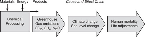
The atmosphere allows solar radiation from the sun to pass through without significant absorption of energy. Some of the solar radiation reaching the surface of the earth is absorbed, heating the land and water. Infrared radiation is emitted from the earth’s surface, but certain gases in the atmosphere absorb this infrared radiation, and re-direct a portion back to the surface, thus warming the planet and making life, as we know it, possible. This process is often referred to as the greenhouse effect. The surface temperature of the earth will rise until a radiative equilibrium is achieved between the rate of solar radiation absorption and the rate of infrared radiation emission. Human activities, such as fossil fuel combustion, deforestation, agriculture and large-scale chemical production, have measurably altered the composition of gases in the atmosphere. Some believe that these alterations will lead to a warming of the earth-atmosphere system by enhancement of the greenhouse effect. Figure 1.4-1 summarizes the major links in the chain of environmental cause and effect for the emission of greenhouse gases.
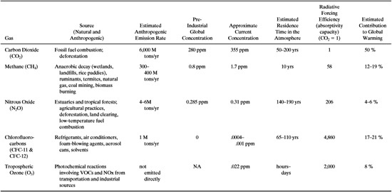
Table 1.4-1 is a list of the most important greenhouse gases along with their anthropogenic (man-made) sources, emission rates, concentrations, residence times in the atmosphere, relative radiative forcing efficiencies, and estimated contribution to global warming. The primary greenhouse gases are water vapor, carbon dioxide, methane, nitrous oxide, chlorofluorocarbons, and tropospheric ozone. Water vapor is the most abundant greenhouse gas, but is omitted because it is generally not from anthropogenic sources. Carbon dioxide contributes significantly to global warming due to its high emission rate and concentration. The major factors contributing to global warming potential of a chemical are infrared absorptive capacity and residence time in the atmosphere. Gases with very high absorptive capacities and long residence times can cause significant global warming even though their concentrations are extremely low. A good example of this phenomenon is the chlorofluorocarbons, which are, on a pound-for-pound basis, more than 1000 times more effective as greenhouse gases than carbon dioxide.
Figure 1.4-1 Greenhouse emission from chemical processes and the major cause and environmental effect chain.
For the past four decades, measurements of the accumulation of carbon dioxide in the atmosphere have been taken at the Mauna Loa Observatory in Hawaii, a location far removed from most human activity that might generate carbon dioxide. Based on the current level of CO2 of 360 parts-per-million (ppm), levels of CO2 are increasing at the rate of 0.5%/year (from about 320 ppm in 1960). Atmospheric concentrations of other greenhouse gases have also risen. Methane has increased from about 700 ppb in pre-industrial times to 1721 ppb in 1994, while N2O rose from 275 to 311 ppb over the same period. While it is clear that atmospheric concentrations of carbon dioxide, and other global warming gases are increasing, there is significant uncertainty regarding the magnitude of the effect on climate that these concentration changes might induce (interested readers should consult the reports of the Intergovernmental Panel on Climate Change (IPCC), see references at the end of the chapter).
1.4.3 Ozone Depletion in the Stratosphere
There is a distinction between “good” and “bad” ozone (O3) in the atmosphere. Tropospheric ozone, created by photochemical reactions involving nitrogen oxides and hydrocarbons at the earth’s surface, is an important component of smog. A potent oxidant, ozone irritates the breathing passages and can lead to serious lung damage. Ozone is also harmful to crops and trees. Stratospheric ozone, found in the upper atmosphere, performs a vital and beneficial function for all life on earth by absorbing harmful ultraviolet radiation. The potential destruction of this stratospheric ozone layer is therefore of great concern.
Table 1.4-1 Greenhouse Gases and Global Warming Contribution. M stands fot million. Phipps (1966), IPCC (1966).
The stratospheric ozone layer is a region in the atmosphere between 12 and 30 miles (20–50 km) above ground level in which the ozone concentration is elevated compared to all other regions of the atmosphere. In this low-pressure region, the concentration of O3 can be as high as 10 ppm (about 1 out of every 100,000 molecules). Ozone is formed at altitudes between 25 and 35 km in the tropical regions near the equator where solar radiation is consistently strong throughout the year. Because of atmospheric motion, ozone migrates to the polar regions and its highest concentration is found there at about 15 km in altitude. Stratospheric ozone concentrations have steadily declined over the past 20 years.
Ozone equilibrates in the stratosphere as a result of a series of natural formation and destruction reactions that are initiated by solar energy. The natural cycle of stratospheric ozone creation and destruction has been altered by the introduction of man-made chemicals. Two chemists, Mario Molina and Sherwood Rowland of the University of California, Irvine, received the 1995 Nobel Prize for Chemistry for their discovery that chlorofluorocarbons (CFCs) take part in the destruction of atmospheric ozone. CFCs are highly stable chemical structures composed of carbon, chlorine, and fluorine. One important example is trichlorofluoromethane, CCl3F, or CFC-11.
CFCs reach the stratosphere due to their chemical properties; high volatility, low water solubility, and persistence (non-reactivity) in the lower atmosphere. In the stratosphere, they are photo-dissociated to produce chlorine atoms, which then catalyze the destruction of ozone (Molina and Rowland, 1974):

The chlorine atom is not destroyed in the reaction and can cause the destruction of up to 10,000 molecules of ozone before forming HCl by reacting with hydrocarbons. The HCl eventually precipitates from the atmosphere. A similar mechanism as outlined above for chlorine also applies to bromine, except that bromine is an even more potent ozone destroying compound. Interestingly, fluorine does not appear to be reactive with ozone. Figure 1.4-2 summarizes the major steps in the environmental cause and effect chain for ozone-depleting substances.
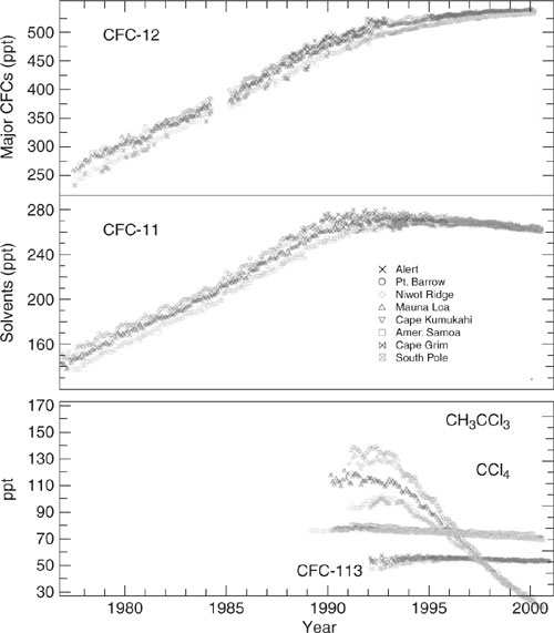
CFC’s were first introduced in the 1930’s for use as refrigerants and solvents. By the 1950’s significant quantities were released into the atmosphere. Releases reached a peak in the mid-eighties (CFC-11 and CFC-12 combined were about 700 million kg). Releases have been decreasing since about 1990 (1995 data: 300 million kg, same level as 1966). The Montreal Protocol, which instituted a phase-out of ozone-depleting chemicals, is the primary reason for the declining trend. Figures 1.4-3 and 1.4-4 show recent trends in the production of several CFCs and in the resulting remote tropospheric concentrations from releases. The growth in accumulation of CFCs in the environment has been halted as a result of the Montreal Protocol.
Figure 1.4-2 Ozone-depleting chemical emissions and the major steps in the environmental cause and effect chain.
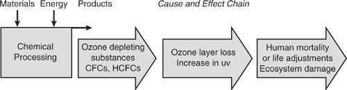
Figure 1.4-3 Recent trends in the production of CFCs and HCFCs. (AFEAS 2000)
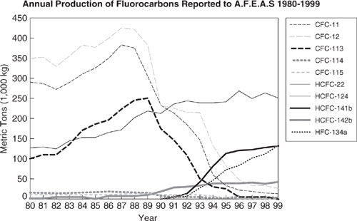
Figure 1.4-4 Trends of controlled ozone-depleting substances under the 1987 Montreal Protocol and its subsequent amendments from the NOAA/CMDL Network. Mixing ratios (dry mole fraction) of CFC-12 are shown in the top panel from flasks except for the 1993-1994 where in situ values are used. Mixing ratios of CFC-11 (collected from flasks) in the middle panel follow the pattern of total equivalent chlorine in the troposphere. Mixing ratios of CH3 CCl3 and CCl4 from in situ measurements and CFC-113 from flask measurements are shown in the bottom panel (updated data from Elkins et al., 1993 and Montzka et al., 1999).
1.5 Air Quality Issues
Air pollution arises from a number of sources, including stationary, mobile, and area sources. Stationary sources include factories and other manufacturing processes. Mobile sources are automobiles, other transportation vehicles, and recreational vehicles such as snowmobiles and watercraft. Area sources are emissions associated with human activities that are not considered mobile or stationary. Examples of area sources include emissions from lawn and garden equipment, and residential heating. Pollutants can be classified as primary, those emitted directly to the atmosphere, or secondary, those formed in the atmosphere after emission of precursor compounds. Photochemical smog (the term originated as a contraction of smoke and fog) is an example of secondary pollution that is formed from the emission of volatile organic compounds (VOCs) and nitrogen oxides (NOx), the primary pollutants. Air quality problems are closely associated with combustion processes occurring in the industrial and transportation sectors of the economy. Smog formation and acid rain are also closely tied to these processes. In addition, hazardous air pollutants, including chlorinated organic compounds and heavy metals, are emitted in sufficient quantities to be of concern. Figure 1.5-1 shows the primary environmental cause and effect chain leading to the formation of smog.
1.5.1 Criteria Air Pollutants
Congress in 1970 passed the Clean Air Act which charged the Environmental Protection Agency (EPA) with identifying those air pollutants which are most deleterious to public health and welfare, and empowered EPA to set maximum allowable ambient air concentrations for these criteria air pollutants. EPA identified six substances as criteria air pollutants (Table 1.5-1) and promulgated primary and secondary standards that make up the National Ambient Air Quality Standards (NAAQS). Primary standards are intended to protect the public health with an adequate margin of safety. Secondary standards are meant to protect public welfare, such as damage to crops, vegetation, and ecosystems or reductions in visibility.
Criteria pollutants are a set of individual chemical species that are considered to have potential for serious adverse health impacts, especially in susceptible populations. These pollutants have established health-based standards and were among the first airborne pollutants to be regulated, starting in the early 1970’s.
Since the establishment of the NAAQS, overall emissions of criteria pollutants have decreased 31% despite significant growth in the U.S. population and economy. Even with such improvements, more than a quarter of the U. S. population lives in locations with ambient concentrations of criteria air pollutants above the NAAQS (National Air Quality Emission Trends Report, www.epa.gov/oar/aqtrnd97/). These criteria pollutants and their health effects will be discussed next.
Figure 1.5-1 Environmental cause and effect chain for photochemical smog formation.

Table 1.5-1 Criteria Pollutants and the National Ambient Air Quality Standards.

1.5.1.1 NOx, Hydrocarbons, and VOCs—Ground-Level Ozone
Ground-level ozone is one of the most pervasive and intractable air pollution problems in the United States. We should again differentiate between this “bad” ozone created at or near ground level (tropospheric) from the “good” or stratospheric ozone that protects us from UV radiation.
Ground-level ozone, a component of photochemical smog, is actually a secondary pollutant in that certain precursor contaminants are required to create it. The precursor contaminants are nitrogen oxides (NOx, primarily NO and NO2) and hydrocarbons. The oxides of nitrogen along with sunlight cause ozone formation, but the role of hydrocarbons is to accelerate and enhance the accumulation of ozone.
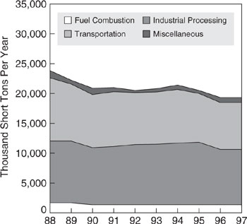
Oxides of nitrogen (NOx) are formed in high-temperature industrial and transportation combustion processes. In 1997, transportation sources accounted for 49.2% and non-transportation fuel combustion contributed 45.4% of total NOx emissions. Health effects associated with short-term exposure to NO2 (less than three hours at high concentrations) are increases in respiratory illness in children and impaired respiratory function in individuals with pre-existing respiratory problems. Figure 1.5-2 shows the NOx emission trends from 1988 to 1997 for major source categories. Industry makes a significant contribution to the “fuel combustion” category from the energy requirements of industrial processes.
Major sources of hydrocarbon emissions are the chemical and oil refining industries, and motor vehicles. In 1997, industrial processes accounted for 51.2% while the transportation sector contributed 39.9% of the total of man-made (nonbiogenic) hydrocarbon sources. Solvents comprise 66% of the industrial emissions and 34% of total VOC emissions. It should be noted that there are natural (biogenic) sources of HCs/VOCs, such as isoprene and monoterpenes that can contribute significantly to regional hydrocarbon emissions and low-level ozone levels. Figure 1.5-3 summarized recent trends in VOC emissions.
Ground-level ozone concentrations are exacerbated by certain physical and atmospheric factors. High-intensity solar radiation, low prevailing wind speed (dilution), atmospheric inversions, and proximity to mountain ranges or coastlines (stagnant air masses) all contribute to photochemical smog formation.
Human exposure to ozone can result in both acute (short-term) and chronic (long-term) health effects. The high reactivity of ozone makes it a strong lung irritant, even at low concentrations. Formaldehyde, peroxyacetylnitrate (PAN), and other smog-related oxygenated organics are eye irritants. Ground-level ozone also affects crops and vegetation adversely when it enters the stomata of leaves and destroys chlorophyll, thus disrupting photosynthesis. Finally, since ozone is an oxidant, it causes materials with which it reacts to deteriorate, such as rubber and latex painted surfaces.
1.5.1.2 Carbon Monoxide (CO)
CO is a colorless, odorless gas formed primarily as a by-product of incomplete combustion. The major health hazard posed by CO is its capacity to bind with hemoglobin in the blood stream and thereby reduce the oxygen-carrying ability of the blood. Transportation sources account for the bulk (76.6%) of total national CO emissions. As noted in Table 1.5-1, ambient CO concentrations have decreased significantly in the past two decades, primarily due to improved control technologies for vehicles. Areas with high traffic congestion generally will have high ambient CO concentrations. High localized and indoor CO levels can come from cigarettes (second-hand smoke), wood-burning fireplaces, and kerosene space heaters.
Figure 1.5-2 Emission trends for major categories of NOx emission sources (US EPA 1998).

Figure 1.5-3 Emission trends for major categories of VOC emission sources (US EPA 1998).
1.5.1.3 Lead
Lead in the atmosphere is primarily found in fine particulates, up to 10 microns in diameter, which can remain suspended in the atmosphere for significant periods of time. Tetraethyl lead ((CH3 CH2)4–Pb) was used as an octane booster and antiknock compound for many years before its full toxicological effects were understood. The Clean Air Act of 1970 banned all lead additives and the dramatic decline in lead concentrations and emissions has been one of the most important yet unheralded environmental improvements of the past twenty-five years. (Table 1.5-1). In 1997, industrial processes accounted for 74.2% of remaining lead emissions, with 13.3% resulting from transportation, and 12.6% from nontransportation fuel combustion (US EPA 1998).
Lead also enters waterways in urban runoff and industrial effluents, and adheres to sediment particles in the receiving water body. Uptake by aquatic species can result in malformations, death, and aquatic ecosystem instability. There is a further concern that increased levels of lead can occur locally due to acid precipitation that increases lead’s solubility in water and thus its bioavailability. Lead persists in the environment and is accumulated by aquatic organisms.
Lead enters the body by inhalation and ingestion of food (contaminated fish), water, soil, and airborne dust. It subsequently deposits in target organs and tissue, especially the brain. The primary human health effect of lead in the environment is its effect on brain development, especially in children. There is a direct correlation between elevated levels of lead in the blood and decreased IQ, especially in the urban areas of developing countries that have yet to ban lead as a gasoline additive.
1.5.1.4 Particulate Matter
Particulate matter (PM) is the general term for microscopic solid or liquid phase (aerosol) particles suspended in air. PM exists in a variety of sizes ranging from a few Angstroms to several hundred micrometers. Particles are either emitted directly from primary sources or are formed in the atmosphere by gas-phase reactions (secondary aerosols).
Since particle size determines how deep into the lung a particle is inhaled, there are two NAAQS for PM, PM2.5, and PM10. Particles smaller than 2.5 m are called “fine,” are composed largely of inorganic salts (primarily ammonium sulfate and nitrate), organic species, and trace metals. Fine PM can deposit deep in the lung where removal is difficult. Particles larger than 2.5 μm are called “coarse” particles, and are composed largely of suspended dust. Coarse PM tends to deposit in the upper respiratory tract, where removal is more easily accomplished. In 1997, industrial processes accounted for 42.0% of the emission rate for traditionally inventoried PM10. Non-transportation fuel combustion and transportation sources accounted for 34.9% and 23.0%, respectively. As with the other criteria pollutants, PM10 concentrations and emission rates have decreased modestly due to pollution control efforts (Table 1.5-1).
Coarse particle inhalation frequently causes or exacerbates upper respiratory difficulties, including asthma. Fine particle inhalation can decrease lung functions and cause chronic bronchitis. Inhalation of specific toxic substances such as asbestos, coal mine dust, or textile fibers are now known to cause specific associated cancers (asbestosis, black lung cancer, and brown lung cancer, respectively).
An environmental effect of PM is limited visibility in many parts of the United States including some National Parks. In addition, nitrogen and sulfur containing particles deposited on land increase soil acidity and alter nutrient balances. When deposited in water bodies, the acidic particles alter the pH of the water and lead to death of aquatic organisms. PM deposition also causes soiling and corrosion of cultural monuments and buildings, especially those that are made of limestone.
1.5.1.5 SO2, NOx, and Acid Deposition
Sulfur dioxide (SO2) is the most commonly encountered of the sulfur oxide (SOx) gases, and is formed upon combustion of sulfur-containing solid and liquid fuels (primarily coal and oil). SOx are generated by electric utilities, metal smelting, and other industrial processes. Nitrogen oxides (NOx) are also produced in combustion reactions; however, the origin of most NOx is the oxidation of nitrogen in the combustion air. After being emitted, SOx and NOx can be transported over long distances and are transformed in the atmosphere by gas phase and aqueous phase reactions to acid components (H2 SO4 and HNO3). The gas phase reactions produce microscopic aerosols of acid-containing components, while aqueous phase reactions occur inside existing particles. The acid is deposited to the earth’s surface as either dry deposition of aerosols during periods of no precipitation or wet deposition of acid-containing rain or other precipitation. There are also natural emission sources for both sulfur and nitrogen-containing compounds that contribute to acid deposition. Water in equilibrium with CO2 in the atmosphere at a concentration of 330 ppm has a pH of 5.6. When natural sources of sulfur and nitrogen acid rain precursors are considered, the “natural” background pH of rain is expected to be about 5.0. As a result of these considerations, “acid rain” is defined as having a pH less than 5.0. Figure 1.5-4 shows the major environmental cause and effect steps for acidification of surface water by acid rain.
Major sources of SO2 emissions are non-transportation fuel combustion (84.7%), industrial processes (8.4%), transportation (6.8%), and miscellaneous (0.1%) (US EPA 1998). As shown in Table 1.5-1, SO2 concentrations and emissions have decreased significantly from 1988 to 1997. Emissions are expected to continue to decrease as a result of implementing the Acid Rain Program established by EPA under Title IV of the Clean Air Act. The goal of this program is to decrease acid deposition significantly by controlling SO2 and other emissions from utilities, smelters, and sulfuric acid manufacturing plants, and by reducing the average sulfur content of fuels for industrial, commercial, and residential boilers.
There are a number of health and environmental effects of SO2, NOx, and acid deposition. SO2 is absorbed readily into the moist tissue lining the upper respiratory system, leading to irritation and swelling of this tissue and airway constriction. Long-term exposure to high concentrations can lead to lung disease and aggravate cardiovascular disease. Acid deposition causes acidification of surface water, especially in regions of high SO2 concentrations and low buffering and ion exchange capacity of soil and surface water. Acidification of water can harm fish populations, by exposure to heavy metals, such as aluminum which is leached from soil. Excessive exposure of plants to SO2 decreases plant growth and yield and has been shown to decrease the number and variety of plant species in a region (USEPA 1998). Figures 1.5-5 shows recent trends in the emission and concentrations of SO2.
Figure 1.5-4 Environmental cause and effect for acid rain.

1.5.2 Air Toxics
Hazardous air pollutants (HAPs), or air toxics, are airborne pollutants that are known to have adverse human health effects, such as cancer. Currently, there are over 180 chemicals identified on the Clean Air Act list of HAPs (US EPA 1998). Examples of air toxics include the heavy metals mercury and chromium, and organic chemicals such as benzene, hexane, perchloroethylene (perc), 1,3-butadiene, dioxins, and polycyclic aromatic hydrocarbons (PAHs).
The Clean Air Act defined a major source of HAPs as a stationary source that has the potential to emit 10 tons per year of any one HAP on the list or 25 tons per year of any combination of HAPs. Examples of major sources include chemical complexes and oil refineries. The Clean Air Act prescribes a very high level of pollution control technology for HAPs called MACT (Maximum Achievable Control Technology). Small area sources, such as dry cleaners, emit lower HAP tonnages but taken together are a significant source of HAPs. Emission reductions can be achieved by changes in work practices such as material substitution and other pollution prevention strategies.
HAPs affect human health via the typical inhalation or ingestion routes. HAPs can accumulate in the tissue of fish, and the concentration of the contaminant increases up the food chain to humans. Many of these persistent and bioaccumulative chemicals are known or suspected carcinogens.
Figure 1.5-5 Emission trends for SO2 from 1988–1997 for different source categories.

1.6 Water Quality Issues
The availability of freshwater in sufficient quantity and purity is vitally important in meeting human domestic and industrial needs. Though 70% of the earth’s surface is covered with water, the vast majority exists in oceans and is too saline to meet the needs of domestic, agricultural, or other uses. Of the total 1.36 billion cubic kilometers of water on earth, 97% is ocean water, 2% is locked in glaciers, 0.31% is stored in deep groundwater reserves, and 0.32% is readily accessible freshwater (4.2 million cubic kilometers). Freshwater is continually replenished by the action of the hydrologic cycle. Ocean water evaporates to form clouds, precipitation returns water to the earth’s surface, recharging the groundwater by infiltration through the soil, and rivers return water to the ocean to complete the cycle. In the United States, freshwater use is divided among several sectors; agricultural irrigation 42%, electricity generation 38%, public supply 11%, industry 7%, and rural uses 2% (Solley et al. 1993). Groundwater resources meet about 20% of U.S. water requirements, with the remainder coming from surface water sources.
Contamination of surface and groundwater originates from two categories of pollution sources. Point sources are entities that release relatively large quantities of wastewater at a specific location, such as industrial discharges and sewer outfalls. Non-point sources include all remaining discharges, such as agricultural and urban runoff, septic tank leachate, and mine drainage. Another contributor to water pollution is leaking underground storage tanks. Leaks result in the release of pollution into the subsurface where dissolution in groundwater can lead to the extensive destruction of drinking water resources.
Besides the industrial and municipal sources we typically think of in regard to water pollution, other significant sources of surface and groundwater contamination include agriculture and forestry. Contaminants originating from agricultural activities include pesticides, inorganic nutrients such as ammonium, nitrate, and phosphate, and leachate from animal waste. Forestry practices involve widespread disruption of the soil surface from road building and the movement of heavy machinery on the forest floor. This activity increases erosion of topsoil, especially on steep forest slopes. The resulting additional suspended sediment in streams and rivers can lead to light blockage, reduced primary production in streams, destruction of spawning grounds, and habitat disruption of fisheries.
Transportation sources also contribute to water pollution, especially in coastal regions where shipping is most active. The 1989 Exxon Valdez oil spill in Prince William Sound in the state of Alaska is a recent well-known case that coated the shoreline with crude oil over a vast area. Routine discharges of petroleum from oil tanker operations is on the order of 22 million barrels per year (UNEP 1991), an amount 87 times the size of the Exxon Valdez spill. Transportation activities can also be a source of non-point pollution as precipitation runoff from roads carries oil, heavy metals, and salt into nearby streams.
1.7 ECOLOGY
Ecology is the study of material flows and energy utilization patterns in communities of living organisms in the environment, termed ecosystems. This area of science is very important in pollution prevention because of the possibility that pollutants entering sensitive ecosystems might disrupt the cycling of essential nutrients and elements for life, with potentially unforeseen negative consequences. Ecosystems, whether aquatic or terrestrial, share a common set of characteristics. They extract energy from the sun and store this energy in the form of reduced carbon-based compounds (biomass) in a process termed photosynthesis. Another very important function of ecosystems is to cycle elements and molecules through the environment, alternating between organic and inorganic forms of carbon, nitrogen, phosphorus, and sulfur.
Organisms that capture solar energy are primary producers which inhabit the first trophic level of the food chain in ecosystems. Examples of primary producers are plants in terrestrial ecosystems. For aquatic systems, members include aquatic plants, algae, and phytoplankton. The second trophic level is inhabited by the primary consumers, such as grazing animals on land and zooplankton and insects in aquatic environments, which prey upon the primary producers. The third trophic level is occupied by the secondary consumers, which prey upon the primary consumers. Examples are birds of prey, mammalian carnivores, fish, and many others. Additional trophic levels are possible depending upon the particular ecosystem.
Carnivores at the highest trophic levels in ecosystem food chains can encounter increased exposure to certain classes of anthropogenic pollutants. Chemicals that are hydrophobic (water-hating, non-polar organic compounds of high molecular weight), persistent (do not biodegrade or react biologically in ecosystems), and toxic are of particular concern because these chemicals bioaccumulate in animal fat tissue and are transferred from lower to higher trophic levels in the food chain. High levels of polychlorinated biphenyls (PCBs), certain pesticides, and mercury compounds have been detected in fish of the Great Lakes. The use of the pesticide DDT in the 1950s and 1960s caused dramatic reductions in birth rates of certain birds of prey that were consuming contaminated fish and other contaminated animals. Such examples demonstrate the need to understand the workings of ecosystems so that one can mitigate the harm that chemicals released into the environment can cause to ecosystems.
1.8 Natural Resources
The production of industrial materials and products begins with the extraction of natural resources from the environment. The availability of these resources is vital for the sustained functioning of both industrialized and developing societies. Examples of natural resources include water, minerals, energy resources like fossil fuels, solar radiation, wind, and lumber. Renewable resources have the capacity to be replenished, while non-renewable resources are only available in finite quantities. The management of natural resources is intended to assure an adequate supply of these materials for anticipated future uses, also known as sustainable use. Non-renewable resources are of particular importance because of their inherently finite supply. For example, most energy requirements of today and of the foreseeable future will be met using non-renewable fossil fuels, such as oil, coal, and natural gas. As the availability of resources is diminished, the costs and energy consumption for producing these materials are likely to increase. Resource management techniques like conservation, recycling of materials, and improved technologies can be used to ensure the availability of these materials for the future. In some cases, materials already in use can be continuously recycled into new products (for instance, lead from batteries, steel from scrap cars, aluminum from beverage cans).
1.9 Waste Flows in the United States
There is no single source of national industrial waste data in the United States. Instead, the national industrial waste generation, treatment, and release picture is a composite derived from several sources of data. A major source of industrial waste data is the United States Environmental Protection Agency, which compiles various national inventories in response to legislative statutes. A sampling of the many laws requiring EPA to collect environmental data include the Clean Air Act, Resource Conservation and Recovery Act (RCRA), Superfund Amendments and Reauthorization Act (SARA), and the Emergency Planning and Community Right-to-Know Act (EPCRA). In addition to these federal government sources of data, there is also information collected by industry consortia such as the American Chemistry Council (formerly the Chemical Manufacturer’s Association) and the American Petroleum Institute. Table 1.9-1 lists a number of national industrial waste databases. Due to the many inventories and the fact that the data sources might contain inconsistent data, the assembly of the national waste picture is difficult. However, from these data sources one is able to identify the major industrial sectors involved and the magnitude of their contributions.
Non-hazardous industrial waste represents the largest contribution to the national industrial waste picture. From 1986 data, almost 12 billion tons of nonhazardous waste was generated and disposed of by U.S. industry (Allen and Rosselot, 1997; US EPA 1988a and 1988b). That amount is about 240 pounds of industrial waste per person each day using today’s population numbers. This amount is about 60 times higher than the rate of waste generation by households in the United States (municipal solid waste). The largest industrial contributors to nonhazardous waste are the manufacturing industry (7,600 million tons/yr), oil and gas industry (2,095–3,609 million tons/yr), and the mining industry (>1,400 million tons/yr). Lesser amounts are contributed by electricity generators (fly ash and flue-gas desulfurization waste), construction waste, hospital infectious waste, and waste tires.
Table 1.9-1 Sources of National Industrial Waste Trends Data. See Appendix F for additional information.
Non-Hazardous Solid Waste |
Report to Congress: Solid Waste Disposal in the United States, Volumes I and II, US Environmental Protection Agency, EPA/530-SW-88-011 and EPA/530-SW-88-011B, 1988. |
Criteria Air Pollutants |
Aerometric Information Retrieval System (AIRS); US EPA Office of Air Quality Planning and Standards, Research Triangle Park, NC. |
National Air Pollutant Emission Estimates; US EPA Office of Air Quality Planning and Standards, Research Triangle Park, NC. |
Hazardous Waste (Air Releases, Wastewater, and Solids) |
Biennial Report System (BRS); available through TRK NET, Washington, DC. |
National Biennial Report of Hazardous Waste Treatment, Storage, and Disposal Facilities Regulated under RCRA; US EPA Office of Solid Waste, Washington, DC. |
National Survey of Hazardous Waste Generators and Treatment, Storage, Disposal and Recycling Facilities in 1986; available through National Technical Information Service (NTIS) as PB92-123025. |
Generation and Management of Residual Materials; Petroleum Refining Performance (replaces The Generation and Management of Wastes and Secondary Materials series); American Petroleum Institute, Washington, DC. |
Preventing Pollution in the Chemical Industry: Five Years of Progress (replaces the CMA Hazardous Waste Survey series); Chemical Manufacturers Association (CMA), Washington, DC. |
Report to Congress on Special Wastes from Mineral Processing; US EPA Office of Solid Waste, Washington, DC. |
Report to Congress: Management of Wastes from the Exploration, Development, and Production of Crude Oil, Natural Gas, and Geothermal Energy, Vol. 1, Oil and Gas; US EPA Office of Solid Waste, Washington, DC. Toxic Chemical Release Inventory (TRI); available through National Library of Medicine, Bethesda, Maryland and RTK NET, Washington, DC. |
Toxic Release Inventory: Public Data Release (replaces Toxics in the Community: National and Local Perspectives); EPCRA hotline (800)-535-0202. www.epa.gov/TRI |
Permit Compliance System; US EPA Office of Water Enforcement and Permits, Washington, DC. |
Economic Aspects of Pollution Abatement |
Manufacturers’ Pollution Abatement Capital Expenditures and Operating Costs; Department of Commerce, Bureau of the Census, Washington, DC. |
Minerals Yearbook, Volume 1 Metals and Minerals; Department of the Interior, Bureau of Mines, Washington, DC. Census Series: Agriculture, Construction Industries, Manufacturers-Industry, Mineral Industries; Department of Commerce, Bureau of the Census, Washington, DC. |
Source: US Department of Energy (DOE), “Characterization of Major Waste Data Sources,” DOE/CE-40762T-H2, 1991. |
Hazardous waste is defined under the provisions of the Resource Conservation and Recovery Act (RCRA) as residual materials which are ignitable, reactive, corrosive, or toxic. Once designated as hazardous, the costs of managing, treating, storing, and disposing of this material increase dramatically. The rate of industrial hazardous waste generation in the United States is approximately 750 million tons/yr (1986 data, Baker and Warren, 1992; Allen and Rosselot, 1997). This rate is 1/16th the rate at which non-hazardous solid waste is generated by industry. Furthermore, hazardous waste contains over 90% by weight of water, having only a relatively minor fraction of hazardous components. Therefore, the rate of generation of hazardous components in waste by industry is estimated at 10–100 million tons/yr, though there is significant uncertainty in the exact amount due to differing definitions of hazardous waste. As shown in Figure 1.9-1, the chemical and allied products industries generate about 51% by weight of the hazardous wastes produced in the United States each year (about 380 million tons/yr on a wet basis). Electronics, petroleum refining and related products, primary metals, and transportation equipment manufacturers each contribute from 50 to 70 million tons/yr.
Releases and waste generation rates for more than 600 chemicals and chemical categories are currently reported to the US EPA in the Toxic Release Inventory (TRI). Manufacturing operations (those with Standard Industrial Classification (SIC) Codes between 20 and 39) and certain federal facilities are required to report their releases of listed chemicals. Facilities must report releases of toxic chemicals to the air, water, and soil, as well as transfers to off-site recycling or treatment, storage, and disposal facilities. The release rate estimates only include the toxic chemicals of any waste stream, thus water or other inerts are not included, in contrast with the industrial hazardous waste reporting system. The total releases and transfers reported to the TRI in 1994 (TRI 1994) was three million tons and the distribution of this amount among several manufacturing categories is shown in Figure 1.9-2. Again, as in hazardous waste, a relatively few industrial sectors release the majority of the toxic pollutants. More recent versions of the TRI have included more industrial sectors (such as electricity generation and mining) in the reporting, resulting in somewhat different distributions. Nevertheless, a few indus-trial sectors continue to dominate the releases.
What happens to all of the hazardous waste generated by the United Stated industry each year? Table 1.9-2 shows several management methods, the quantity of hazardous waste managed, and the number of facilities involved. Note that the quantities managed in Table 1.9-2 add up to more than 750 million tons/year because the same waste may be counted in more than one management method. For example, some wastewater may be stored or may be temporarily placed in surface impoundments before treatment. It is also interesting to note that 96% of hazardous wastes are managed on-site at the facilities that generated them in the first place. Most hazardous waste is managed using wastewater treatment. This is not surprising because over 90% of hazardous waste is water. Also, very little recycling and recovery of hazardous waste components occurs.
Figure 1.9-1 Industrial hazardous waste generation in the United States by industry sector (1986 data, Baker and Warren, 1992).
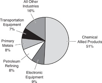
Figure 1.9-2 Adapted from Allen and Rosselot, 1997. Toxic chemical releases from United States industry as a percentage of the total release (3 million tons per year). Source: Allen and Rosselot, Pollution Prevention for Chemical Processes xs© 1997. This material is used by permission of John Wiley & Sons, Inc.

Table 1.9-2 Hazardous Waste Managed for Each Management Technology (1986 data).

Summary
In this chapter a wide array of environmental issues were introduced, and their impacts were related to chemical production and use. The pertinent chemicals and the environmental reactions of those chemicals were discussed. For many environmental problems, the chemicals causing the adverse environmental or health impacts were not the same chemical originally emitted from the production process or from the use of a chemical. Thus, the environment is a complex system with a large number of transport and transformation processes occurring simultaneously. Fortunately for the chemical engineer, it is not necessary to understand these processes in great detail in order to gain the insights needed to design chemical processes to be more efficient and less polluting. A focal point for improving process designs is to understand that the properties of chemicals can have an important influence on their ultimate fate in the environment and on their potential impact on the environment and human health. The influences of chemical properties on how chemicals may behave in the environment will be discussed in detail in Chapters 5 and 6. With a basic understanding of environmental issues, the chemical engineer will be able to spot environmental problems earlier and will contribute to the solution of those problems by improving the environmental performance of chemical processes and products.
References
AFEAS, Alternative Fluorocarbons Environmental Acceptability Study, 1333 H Street NW, Washington, DC 20005 USA, http://www.afeas.org/. Sept. 2000.
Allen, D.T. and Rosselot, K.S., Pollution Prevention for Chemical Processes, John Wiley and Sons, New York, NY, 1997.
Baker, R.D. and Warren, J.L., “Generation of hazardous waste in the United States,” Hazardous Waste & Hazardous Materials, 9(1), 19–35, Winter 1992.
EIA, Energy Information Agency, International Energy Outlook 1998, US Department of Energy, DOE/EIA-0484(98), April 1998a.
EIA, Energy Information Agency, Annual Energy Review, U.S. Department of Energy, DOE/EIA-0484(98), July 1998b.
Elkins, J.W., Thompson, T.M., Swanson, T.H., Butler, J.H., Hall, B.D., Cummings, S.O., Fisher, D.A., and Raffo, A.G., Decrease in the growth rates of atmospheric chlorofluorocarbons 11 and 12, Nature, 364, 780–783, 1993.
IPCC, Intergovernment Panel on Climate Change, Climate Change 1995: The Science of Climate Change, ed. Houghton, J.T., Milho, L.G.M., Callander, B.A., Harris, H. Kattenberg, A., and Maskell, K., Cambridge University Press, Cambridge, UK, 1996.
Molina, M.J. and Rowland, R.S. “Stratospheric sink for chlorofluoromethanes: Chlorine atom-catalyzed destruction of ozone,”Nature, V. 249: 810–812 (1974).
Montzka, S.A., Butler, J.H., Elkins, J.W., Thompson, T.M., Clarke, A.D., and Lock, L.T., Present and future trends in the atmospheric burden of ozone-depleting halogens, Nature, 398, 690–694, 1999.
NOAA, National Oceanic and Atmospheric Administration, Climate Monitoring and Diagnostics Laboratory, Boulder, CO, http://www.cmdl.noaa.gov/, September 2000.
Phipps, E., Overview of Environmental Problems, National Pollution Prevention Center for Higher Education, University of Michigan, Ann Arbor, MI, 1996, http://www.css.snre.umich.edu
Solley, W.B., Pierce, R.R., and Perlman, H.A., Estimated Use of Water in the United States 1990, US Geological Survey Circular 1081 (Washington: Government Printing Office, 1993).
TRI94, Toxic Chemical Release Inventory for 1994, Bethesda, MD, National Library of Medicine, July 1996.
UNEP, United Nations Environment Programme, The State of The World Environment: 1991, 37, May 1991.
US EPA, United States Environmental Protection Agency, “Report to Congress: Solid Waste Disposal in the United States, Volume 1,” EPA/530-SW-88-011, 1988a.
US EPA, United States Environmental Protection Agency, “Report to Congress: Solid Waste Disposal in the United States, Volume 1,” EPA/530-SW-88-011B, 1988b.
US EPA, United States Environmental Protection Agency, 1997 National Air Quality and Emissions Trends Report, Office of Air Quality Planning and Standards, Research Triangle Park, NC 27711, EPA 454/R-98-016, December 1998, http://www.epa.gov/oar/aqtrnd97/.
Wallace, J.M. and Hobbs, P.V., Atmospheric Science: An Introductory Survey, Academic Press, New York, NY, 1977.
WEC, World Energy Council, Energy for Tomorrow’s World, St. Martin’s Press, New York, NY, pg. 111, 1993.
Problems
1. Electric Vehicles: Effects on Industrial Production of Fuels. Replacing automobiles having internal combustion engines with vehicles having electric motors is seen by some as one solution to urban smog and tropospheric ozone. Write a short report (1–2 pages double spaced) on the likely effects of this transition on industrial production of fuels. Assume for this analysis that the amount of energy required per mile traveled is roughly the same for each kind of vehicle. Consider the environmental impacts of using different kinds of fuel for the electricity generation to satisfy the demand from electric vehicles. This analysis does not include the loss of power over the lines/grid. Background reading for this problem is found in Industrial Ecology and the Automobile by Thomas Graedel and Braden Allenby, Prentice Hall, 1998.
2. Global Energy Balance: No Atmosphere (adapted from Wallace and Hobbs, 1977). The figure below is a schematic diagram of the earth in radiative equilibrium with its surroundings assuming no atmosphere. Radiative equilibrium requires that the rate of radiant (solar) energy absorbed by the surface must equal the rate of radiant energy emitted (infrared). Let S be the incident solar irradiance (1,360 Watts/meter2),E the infrared planetary irradiance (Watts/meter2), RE the radius of the earth (meters), and A the planetary albedo (0.3). The albedo is the fraction of total incident solar radiation reflected back into space without being absorbed.
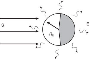
(a) Write the steady-state energy balance equation assuming radiative equilibrium as stated above. Solve for the infrared irradiance, E, and show that its value is 238 W/meter2.
(b) Solve for the global average surface temperature (K) assuming that the surface emits infrared radiation as a black body. In this case, the Stefan-Boltzman Law for a blackbody is E = σ T4, σ is the Stefan-Boltzman Constant (5.67×10⁻⁸ Watts/(m2•°K4)), and T is absolute temperature (°K). Compare this temperature with the observed global average surface temperature of 280 K. Discuss possible reasons for the difference.
3. Global Energy Balance: with a Greenhouse Gas Atmosphere (adapted from Wallace and Hobbs, 1977). Refer to the schematic diagram below for energy balance calculations on the atmosphere and surface of the earth. Assume that the atmosphere can be regarded as a thin layer with an absorbtivity of 0.1 for solar radiation and 0.8 for infrared radiation. Assume that the earth surface radiates as a black body (absorbtivity = emissivity = 1.0).
Let x equal the irradiance (W/m2) of the earth surface and y the irradiance (both upward and downward) of the atmosphere. E is the irradiance entering the earth-atmosphere system from space averaged over the globe (E = 238 W/m2 from problem 2). At the earth’s surface, a radiation balance requires that

0.9E + y = x
(irradiance in irradiance out)
while for the atmosphere layer, the radiation balance is
E + x = 0.9E + 2y + .2x
(a) Solve these equations simultaneously for y and x.
(b) Use the Stefan-Boltzman Law (see problem 2) to calculate the temperatures of both the surface and the atmosphere. Show that the surface temperature is higher than when no atmosphere is present (problem 2).
(c) The emission into the atmosphere of infrared absorbing chemicals is a concern for global warming. Determine by how much the absorbtivity of the atmosphere for infrared radiation must increase in order to cause a rise in the global average temperature by 1° C above the value calculated in part b.
4. Global Carbon Dioxide Mass Balance. Recent estimates of carbon dioxide emission rates to and removal rates from the atmosphere result in the following schematic diagram (EIA, 1998a)
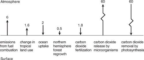
The numbers in the diagram have units of 109 metric tons of carbon per year, where a metric ton is equal to 1000 kg. To calculate the emission and removal rates for carbon dioxide, multiply each number by the ratio of molecular weights (44 g CO2/12 g C).
(a) Write a steady state mass balance for carbon dioxide in the atmosphere and calculate the rate of accumulation of CO2 in the atmosphere in units of kg/yr. Is the accumulation rate positive or negative?
(b) Change the emission rate due to fossil fuel combustion by 10% and recalculate the rate of accumulation of CO2 in the atmosphere in units of kg/yr. Compare this to the change in the rate of accumulation of CO2 in the atmosphere due to a 1% change in carbon dioxide release by micro-organisms.
(c) Calculate the rate of change in CO2 concentration in units of ppm per year, and compare this number with the observed rate of change stated in section 1.4.2. Recall the definition of parts per million (ppm), which for CO2, is the mole fraction of CO2 in the air. Assume that we are only considering the first 10 km in height of the atmosphere and that its gases are well mixed. Take for this calculation that the total moles of gas in the first 10 km of the atmosphere is approximately 1.5×10²⁰ moles.
(Note: ![]() , where Cco2 is the number of moles of CO2 and C is the total moles of air.)
, where Cco2 is the number of moles of CO2 and C is the total moles of air.)
(d) Describe how the rate of accumulation of CO2 in the atmosphere, calculated in parts b and c, would change if processes such as carbon dioxide fertilization and forest growth increase as CO2 concentrations increase. What processes releasing CO2 might increase as atmospheric concentrations increase? (Hint: assume that temperature will rise as CO2 concentrations rise).
5. Ozone Depletion Potential of Substitute Refrigerants. A chemist is trying to develop new alternative refrigerants as substitutes for chlorofluorocarbons. The chemist decides that either bromine or fluorine will substitute for the chlorines on existing compounds. Which element, bromine or fluorine, would be more effective in reducing the ozone depletion potential for the substitute refrigerants? Explain your answer based on the information contained in this chapter.