
Chapter 12
Environmental Cost Accounting
12.1 Introduction
Costs associated with poor environmental performance can be devastating. Waste disposal fees, permitting costs, and liability costs can all be substantial. Wasted raw material, wasted energy and reduced manufacturing throughput are also consequences of wastes and emissions. Corporate image and relationships with workers and communities can suffer if environmental performance is substandard. But, how can these costs be quantified?
This chapter will review the tools available for estimating environmental costs. Many of these tools are still in their developmental stages, and practices therefore vary widely from company to company. In general, however, traditional accounting practices have acted as a barrier to implementation of green engineering projects because they hide the costs of poor environmental performance. Many companies are now giving more consideration to all significant sources of environmental costs. The principle is that if costs are properly accounted for, business management practices that foster good economic performance will also foster superior environmental performance.
The relationships between economic and environmental performance are examined in a number of steps. First, in Section 12.2, a few key terms are defined to simplify and clarify the presentation of material. In Section 12.3, the magnitude and types of environmental costs typically encountered by companies are reviewed. Then, in Section 12.4, a framework for assessing environmental costs is described. Finally, Sections 12.5 through 12.8 describe specific methods for evaluating environmental costs.
Prerequisites to fully understanding the benefits of environmental accounting practices are an understanding of the time value of money and some familiarity with present value, payback period, internal rate of return, and other financial evaluation calculations. These concepts are covered in textbooks on engineering economics (see, for example, Valle-Riestra, 1983). Also, it is assumed that the reader understands how to evaluate potential environmental impacts associated with products and processes (see Chapter 11).
12.2 Definitions
Environmental accounting is still in its infancy and terminology is therefore continually evolving. Precise definitions of terms are often elusive. Nevertheless, to keep the discussion presented in this chapter clear, it is useful to define a number of terms as they will be used in this text. Many of these definitions are drawn from an introduction to environmental accounting prepared by the US Environmental Protection Agency (US EPA, 1995).
Internal costs, or private costs, are costs that are borne by a facility. Costs for materials and labor are examples of internal costs. External costs, or societal costs, on the other hand, are the costs to society of the facility’s activities. The cost associated with a loss of fishable waters due to pollutants discharged by a facility to a stream is an example of an external cost. Often, environmental fees, regulations, and requirements act to internalize what would have otherwise been an external cost, so that a facility that produces waste must pay to reduce its quantity or toxicity or pay a premium for its disposal. This chapter focuses primarily on internal costs.
There are two types of accounting that are pursued at most large facilities: management accounting and financial accounting. Management accounting is the collection of information that helps a firm to make internal decisions. This information is not usually disclosed to the public, and each firm has its own style and accounting requirements. Green accounting (accounting that promotes environ-mentally sound practices) refers to managerial accounting practices. Financial accounting, in contrast, is the information collected for reporting to stockholders, the Securities and Exchange Commission (which oversees trade and investment practices of companies in the United States), and banks. Financial accounting practices tend to be fairly uniform across companies and are governed by generally accepted accounting principles.
A typical management accounting system for a manufacturer would include categories for direct materials and labor (costs that are clearly and exclusively associated with a product or service), manufacturing overhead, sales, general and ad-ministrative overhead, and research and development. Environmental expenses can be hidden in any or all of these categories, but are charged most often as overhead. Overhead costs, as opposed to costs of direct materials and labor for production, are often referred to as indirect costs and consist of any costs that the accounting system either pools facility-wide and does not allocate among activities, or that are allocated on the basis of a formula. Overhead generally includes indirect materials and labor, capital depreciation, rent, property taxes, insurance, supplies, utilities, and repair and maintenance. It can also include labor costs ranging from supervisor salaries to janitorial services. Often, even the direct environmental costs that could be assigned to a particular process, product, or activity, such as waste disposal, are lumped together facility-wide. This is often done because of practices such as using a single waste disposal company to manage all of a facility’s waste. Other environmental costs, such as the costs of filling out forms for reporting waste management practices, are also hidden in the overhead category. Because environmental costs are not traditionally allocated to the activity that is generating wastes, some of the benefits of green engineering projects are masked.
Full-cost accounting is a type of managerial accounting that is considered to be “green.” In full-cost accounting, as many costs as possible are allocated to product, product lines, processes, services, or activities. Full-cost accounting is not a strictly environmental activity. For instance, it is pursued because it is useful in determining the profitability of processes and products and in setting prices. Even though full-cost accounting does not focus particularly on environmental costs, it promotes improved environmental performance because the costs of producing waste for individual processes or products are revealed, providing management with a better idea of the true costs associated with the generation of wastes and emissions.
Activity-based costing is similar to full-cost accounting except that the costs are allocated to specific measures of activity. For example, in activity-based costing, the cost of generating a particular kind of waste per pound of production might be measured. Another example would be determining the cost of chemical inputs per item for painting.
Capital is the wherewithal a facility has to produce goods or to bring in income. Capital budgeting, sometimes called investment analysis or financial evaluation, is supported by information from accounting activities. Each firm has its own capital budgeting process for making decisions about how capital will be spent. How a firm employs the standard evaluation measures such as rate of return, payback period, or net present value, to analyze potential products is individualized. In addition, each firm has self-defined hurdles for determining which projects are worthwhile. For example, for firms using rate of return to evaluate projects, the minimum internal rate of return required to fund a project varies from one company to the next, as do techniques for estimating future interest and inflation rates.
Total cost assessment, discussed in more detail later, is a capital budgeting procedure that requires a comprehensive analysis of savings and costs (especially environmental costs and savings) beyond the capital and operating costs that are conventionally considered in capital budgeting. Life-cycle costing is another type of capital budgeting in which the costs of a project from its conception (e.g., the research and development phase) to its retirement (e.g., salvage value) are assessed. Note that in this chapter, life-cycle costing is assumed to include only internal costs and is not to be confused with life-cycle assessment, which is the assessment of the environmental impacts of a product, process, or activity from raw material extraction to final disposal (see Chapter 13). Life-cycle costing affects decisions about capital expenditure because replacement and closure costs (also called back-end or exit costs) are often hidden, as are up-front costs like research and development.
These are the primary terms that will be used in this chapter. It is useful to keep in mind that precise definitions remain in flux, and vary from organization to organization, so the terminology used in this chapter is not universal. Nevertheless, it is generally recognized that in environmental accounting, words like “full” (e.g., full-cost accounting), “total” (e.g., total cost assessment), and “life-cycle” (e.g., life-cycle costing) are used to indicate that not all costs are captured in traditional accounting and capital budgeting practices.
12.3 Magnitudes of Environmental Costs
The definitions in the previous section made clear that not all environmental costs are captured in traditional accounting and capital budgeting practices. Nevertheless, some measures of environmental costs are available, providing a rough indication of the magnitude of environmental costs and the variation of those costs among industry sectors.
Among the easiest environmental costs to track are the costs associated with treating emissions and disposing of wastes. Direct costs of pollution abatement are tracked by the U.S. Census Bureau, and have been increasing steadily. Expenditures in 1972 totaled $52 billion (in 1990 dollars) and have been projected to grow to approximately $140 billion (1990 dollars), or 2.0-2.2% of Gross National Product, in the year 2000 (for a review and analysis of these data, see US Congress, Office of Technology Assessment, 1994).
Table 12.3-1 Pollution Abatement Expenditures by U.S. Manufacturing Industries (data reported by US Congress, Office of Technology Assessment, 1994; original data collected by U.S. Census Bureau).
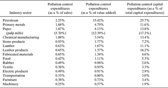
These expenditures are not distributed uniformly among industry sectors. As shown in Table 12.3-1, sectors such as petroleum refining and chemical manufacturing spend much higher fractions of their net sales and capital expenditures on pollution abatement than other industrial sectors. Therefore, in these industrial sectors, minimizing costs by preventing wastes and emissions will be far more strategic an issue than in other sectors.
Table 12.3-2 Summary of Environmental Costs at the Amoco Yorktown Refinery (Heller, et al., 1995).
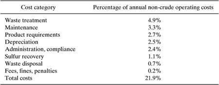
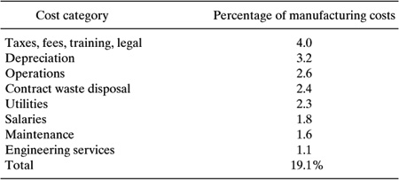
Table 12.3-3 Summary of Environmental Costs at the DuPont LaPorte Chemical Manufacturing Facility (Shields, et al., 1995).
Pollution abatement costs reported by individual companies both reflect these general trends and provide more detail about the magnitude and the distribution of environmental expenditures. For example, Tables 12.3-2 and 12.3-3 show the distribution of environmental costs reported by the Amoco Yorktown refinery and DuPont’s LaPorte chemical manufacturing facility (Heller, et al., 1995; Shields, et al., 1995). In the case of the Amoco refinery, only about a quarter of the quantified environmental costs are associated with waste treatment and disposal—the costs summarized in Table 12.3-2. Costs associated with removing sulfur from fuels, meeting other environmentally-based fuel requirements and maintaining environmental equipment were greater than the costs associated with waste treatment and disposal. This indicates that the magnitude of environmental costs is substantially greater than that reported in Table 12.3-2 —and that these costs may be hard to identify.
Table 12.3-3 shows that the profile of environmental costs at a DuPont chemical manufacturing facility exhibits many of the same characteristics. Waste treatment and disposal costs are less than a quarter of the annual, quantifiable, environmental costs.
Taken together, Tables 12.3-1 through 12.3-3 demonstrate that environmental costs are substantial, but that quantifying these costs is challenging. The next several sections of this chapter present a framework and procedures for estimating these costs.
12.4 A Framework For Evaluating Environmental Costs
Engineering projects are generally not undertaken unless they are financially justifiable. Projects designed to improve environmental performance beyond regulatory requirements usually must compete financially with all other projects under consideration at a facility. Fortunately, improved environmental performance is frequently profitable. Since the potential profitability of environmental projects is difficult to assess, it is common to neglect many of the financial benefits of improved environmental performance when projects are analyzed. That is why a better understanding of methods for estimating environmental costs and benefits serves to promote green engineering.
In this section, the types and magnitudes of costs associated with emissions and waste generation are described and categorized. Five categories, or tiers, of costs will be considered, following the framework recommended in the Total Cost Assessment Methodology developed by the American Institute of Chemical Engineers’ Center for Waste Reduction Technologies (AIChE CWRT, 2000; see Appendix F). The tiers are:
• Tier I—Costs normally captured by engineering economic evaluations.
• Tier II—Administrative and regulatory environmental costs not normally assigned to individual projects.
• Tier III—Liability costs.
• Tier IV—Costs and benefits, internal to a company, associated with improved environmental performance.
• Tier V—Costs and benefits, external to a company, associated with improved environmental performance.
Tier I costs are the types of costs quantified in traditional economic analyses. Specific examples are provided in Table 12.4-1. As discussed in Sections 12.1 through 12.3, traditional accounting systems that focus on Tier I costs fail to capture some types of environmental costs. Examples of some of the costs that are frequently overlooked by traditional methods are listed in Table 12.4-2.
The costs listed in Table 12.4-2 are generally charged to overhead and therefore may be “hidden” when project costs are evaluated. These will be referred to as Tier II or hidden costs. Note that these costs are actually borne by facilities regardless of whether facilities choose to quantify them or assign them to project or product lines.
A less tangible set of costs are those designated as Tier III—liability costs. An accounting definition of liability is a “probable future sacrifice of economic benefits arising from present obligations to transfer assets or provide services in the future”
Table 12.4-1 Costs that are traditionally evaluated during financial analyses of projects.
• Capital equipment |
Table 12.4-2 Environmental costs that are often charged to overhead.
• Off-site waste management charges |
• Waste treatment equipment |
• Waste treatment operating expenses |
• Filing for permits |
• Taking samples |
• Filling out sample reporting forms |
• Conducting waste and emission inventories |
• Filling out hazardous waste manifests |
• Inspecting hazardous waste storage areas and keeping logs |
• Making and updating emergency response plans |
• Sampling stormwater |
• Making chemical usage reports (some states) |
• Reporting on pollution prevention plans and activities (some states) |
(Financial Accounting Standards Board Concept Statement No. 6, Paragraph 35 (1985); Institute of Management Accountants Statement No. 2A Management Accounting Glossary (1990)). Liability costs could include:
• Compliance obligations
• Remediation obligations
• Fines and penalties
• Obligations to compensate private parties for personal injury, property damage, and economic loss
• Punitive damages
• Natural resource damages
A final set of costs are designated as Tier IV or Tier V, which can be referred to as image or relationship costs (AIChE CWRT, 2000). These costs arise in relationships with customers, investors, insurers, suppliers, lenders, employees, regulators, and communities. They are perhaps the most difficult to quantify.
Thus, a basic framework for estimating costs and benefits associated with environmental activities consists of 5 tiers, beginning with the most tangible costs and extending to the least quantifiable costs. The remaining sections of this chapter will focus on methods for estimating Tier II, III, IV, and V costs. Tier I costs, by definition, are captured effectively by conventional accounting methods and are described in detail in texts on engineering economics (see, for example, Valle-Riestra, 1983). The description of Tier II costs in Section 12.5 focuses on methods for quantifying reporting, notification, and compliance costs. These are costs that are certain, yet are often difficult to separate from general overhead expenditures.
Estimating Tier III, IV, and V costs poses different challenges. These costs are often due to unplanned events, such as incidents that result in civil fines, remediation costs, or other charges. While these events are not planned, they do occur, and it is prudent to estimate the expected value of these costs. Arriving at an expected value for Tier III, IV, and V costs will involve estimating three distinct parameters:
1. The probability that an event will occur.
2. The costs associated with the event.
3. When the event will occur.
For example, if the goal is to estimate the expected value of a civil fine or penalty (a Tier III cost), the likelihood that a fine will be assessed and the likely magnitude of that fine must be calculated. If the probability of a fine being assessed is 0.1 (1 chance in 10) per year and the likely magnitude of the fine is $10,000, the expected annual cost due to fines would be $1000. For events that will occur in future years, such as costs of complying with anticipated future regulations, knowledge of when the event will occur is critical to determining the present value of the expected costs. These estimation methods are described in Sections 12.6 through 12.8.
12.5 Hidden Environmental Costs
Table 12.4-2 described a number of emission and waste management charges that are frequently viewed as overhead costs, and therefore can be overlooked by traditional accounting systems. These charges can be grouped into a number of broad categories, specifically waste treatment costs, regulatory compliance costs, and hidden capacity costs.
Waste treatment costs are the most straightforward to estimate. They are frequently hidden because many facilities charge the capital and operating costs of centralized air and water treatment facilities to overhead, rather than to specific processes. Specific treatment costs will vary from facility to facility and will depend strongly on the types of pollutants being treated. However, order-of-magnitude estimates of treatment costs can be estimated using values suggested by Douglas and co-workers (Schultz, 1998), as shown in Table 12.5-1.
Table 12.5-1 Order-of-Magnitude Estimates of Treatment Costs Developed by Douglas and Co-workers (Schultz, 1998).

Example 12.5-1 (Adapted from Schultz, 1998)
A preliminary process design for a process to produce Bis (2-Hydroxyethyl) Terephthalate (BHET) from oxygen, ammonia, xylene and ethylene glycol results in the following estimates of raw material requirements and waste generation:
Raw Materials per mole of BHET (Molecular weight (MW) =254)
1 mole para-xylene (MW=106; cost=$0.40/lb)
2 moles ammonia (MW=17; cost=$0.065/lb)
2 moles ethylene glycol (MW=62; cost=$0.176/lb)
3+ moles oxygen (derived from air—no material acquisition cost)
Wastes generated per pound of product
3.17 pounds of gaseous effluent to be treated
0.39 pound of water to be treated
0.01 pound of organic solid waste to be incinerated
Provide a preliminary estimate of waste treatment costs and compare these to raw material costs per pound of product.

The waste disposal operating costs are:
3.17 * $0.00015 + 0.39*$0.000074 + 0.01*$0.80 = $0.0085 per pound
The costs total about 3% of raw material costs (reasonably consistent with the data presented in Section 12.3) and are dominated by the costs of incineration.
A second major category of hidden environmental costs are the personnel costs associated with meeting environmental regulations. These costs are difficult to account for because environmental reporting and recordkeeping is frequently performed by corporate staff who divide their time between many different processes and facilities. Nevertheless, it is possible to estimate the time required to meet notification, reporting, manifesting, and other administrative tasks associated with environmental record keeping. Appendix E contains worksheets that can be used for this purpose.
Finally, two major costs associated with waste generation that are frequently overlooked are lost raw materials and lost capacity. As an example, consider a process that converts raw material A into product P and waste W. If the yield for the process is increased from 90% to 95%, waste generation and therefore waste disposal costs are cut in half. Not as obvious, however, is the fact that for a given quantity of raw material, the yield of product has increased by 5.5% (5% increase in yield/90% base yield). Further, the same processing equipment (reactors) are able to increase production, and the costs for separating product from wastes may decrease dramatically. Savings due to increased production capacities and increased use of raw materials can often be more substantial than avoided treatment costs.
A chemical manufacturing facility buys raw material for $0.50 per pound and produces 90 million pounds per year of product, which is sold for $0.75 per pound. The process is typically run at 90% selectivity and the raw material that is not converted into product is disposed of at a cost of $0.80 per pound (by incineration). A process improvement allows the process to be run at 95% selectivity, allowing the facility to produce 95 million pounds per year of product. What is the net revenue of the facility (product sales - raw material costs - waste disposal costs) before and after the change? How much of the increased net revenue is due to increased sales of product and how much is due to decreased waste disposal costs?
Solution: The net revenue before the change is:
![]()
The net revenue after the change is:
![]()
Of the difference ($7.75 million), about half ($3.75 million) is due to increased product sales and the remainder is due to decreased disposal cost. Note that the disposal cost assumed in this example is very high and thus represents a likely upper bound on these costs. It should also be noted that the cost of capital depreciation per pound of product is reduced after the change.
12.6 Liability Costs
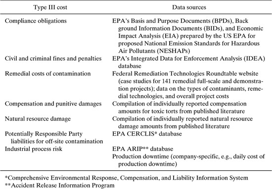
Tier III (liability) costs include future compliance costs and compliance obligations, potential civil and criminal fines and penalties, potential remedial costs of contamination, potential compensation and punitive damages, potential judgements for natural resource damage, Potentially Responsible Party (PRP) liabilities for off-site contamination, and potential industrial process risk. Estimation methodologies for each of these costs have been developed through the AIChE’s Center for Waste Reduction Technologies (AIChE CWRT, 2000) using the data described in Table 12.6-1. A summary of most of the available estimation methodologies has been assembled by the US EPA (US EPA, 1996).
It is beyond the scope of this chapter to describe the methodologies for estimating all of these costs. (See Appendix F for sources of additional information.) Instead, since the procedures for estimating the costs in each of the categories are similar, our focus will be on the procedures. The procedures will be illustrated by considering the cost categories of civil and criminal fines and penalties, and Potentially Responsible Party liabilities for off-site contamination.
Table 12.6-1 Sources of Data Used in AIChE CWRT Total Cost Assessment Methodology (AIChE CWRT, 2000).
In each case, arriving at an expected value of the liability cost will involve estimating three parameters:
1. The probability that an event will occur.
2. The costs associated with the event.
3. When the event will occur.
Consider first the cost category of civil and criminal fines and penalties. Even the best-run manufacturing facilities have occasional violations of environmental statutes. These might be violations due to inadequate reporting or notification (often called paperwork violations), or violations due to process upsets. Most companies keep historical records of these violations, and these can be used to estimate the probability of future fines and penalties. In estimating the probability of a fine or penalty, it should be recognized that not all process units are equally likely to be fined. Factors influencing the probability of a fine or penalty include (AIChECWRT, 2000):
• The extent that spill control measures will be in place.
• The history and reputation of the plant or company.
• The local culture and visibility of the operation to non-governmental organizations.
• How well the administrative requirements of monitoring, recording, and recordkeeping will be maintained.
• The toxicity of the potential contaminants.
• The chance for a large release.
Because probabilities of fines and penalties can vary widely from company to company, this section will assume that these probabilities are known, either through company data or through estimates based on information assembled by the CWRT (AIChE CWRT, 2000).
Estimated magnitudes of fines and penalties vary by statute, as shown in Table 12.6-2. They also vary greatly in magnitude within a given governing statute. For example, most civil fines under the Safe Drinking Water Act are under $20,000, but the largest fines can be as high as $2,500,000. This skewed distribution results in large differences between average and median values for fines and penalties.
Example 12.6-1 illustrates how probabilities of occurrence can be combined with estimated costs to lead to an expected value of civil fine and penalties.
Table 12.6-2 Summary of Penalty Data Assembled for the Total Cost Accounting Methodology of the AIChE CWRT (AIChE CWRT, 2000).

Example 12.6-1
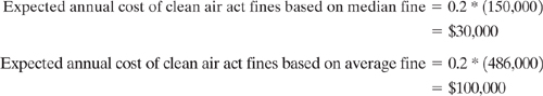
A manufacturing facility operates under an air permit and generates an industrial hazardous waste. The facility has a good record of compliance with air regulations (1 violation in the past 5 years due to a release during an emergency shutdown) and has had two violations under RCRA during the past five years—both due to improper completion of hazardous waste manifest reports. Estimate the annual costs due to civil and administrative fines and penalties.
Solution: Based on the historical data, the probability of an air release resulting in a fine is 0.2/year. If these releases are due to an emergency shutdown and the emergency release is properly reported, an administrative fine, rather than a civil fine, might be anticipated. The expected value of this cost could be calculated using either the average or median value of administrative fines under the Clean Air Act.
Expected annual cost of clean air act fines based on median fine=0.2*(10,000)=$2,000
Expected annual cost of clean air act fines based on average fine=0.2*(21,000)= $4,000
In contrast, if the violation resulted in a civil fine the expected costs would be:
Again, based on historical data, the annual probability of a violation of RCRA is 0.4. Assuming that a paperwork violation would result in an administrative fine, the expected cost would be:
Expected annual cost of RCRA fines based on median fine=0.4*(1,000)=$400
Expected annual cost of RCRA fines based on avereage fine=0.4*(31,000)=$12,000
The range of costs calculated in this example point out that fines and penalties can either be relatively minor costs or they can be major costs. The range of values highlights the importance of collecting company-specific data in estimating likely fines and penalties.
Consider next another category of Tier III costs, Potentially Responsible Party liabilities for off-site contamination. These costs arise when a facility is identified as responsible for site contamination, and therefore must bear the cost of remediating the site. The probability of a remediation cost occurring is, of course, strongly dependent on the practices used in managing wastes and emissions. Company-specific data should be used whenever possible in estimating these probabilities. Again, this section will assume that these probabilities are known, either through company data or through estimates based on information assembled by the CWRT (AIChE CWRT, 2000).
The magnitude of remediation liabilities can be large, as shown in Table 12.6-3, and can depend on a number of factors, including
• the number of responsible parties at the site
• the volume of waste disposed at the site relative to other parties
• the toxicity of the contaminants
• future use of the site
Again, the costs can vary greatly in magnitude and the skewed nature of the cost distribution results in large differences between average and median values for fines and penalties. Example 12.6-2 illustrates how these data might be used to arrive at expected values for remediation costs.
Table 12.6-3 Typical Remediation Costs (AIChE CWRT, 2000).

Example 12.6-2
A manufacturing facility generates an industrial hazardous waste and sends that waste to a landfill. In order to anticipate future remediation costs, the company collects data on the number of remediation actions with which operators of similar disposal sites have been associated. The data indicate that on average, none of the similar sites have required remediation after 5 years of operation, 10% of similar disposal sites have required groundwater remediation after 10 years of operation and 30% of similar sites have required groundwater remediation after 15 years of operation.
The landfill that the facility uses has been in operation for five years and is used in roughly equal amounts by 5 manufacturing facilities. Estimate the expected remediation costs over the next 10 years.
Solution: Based on the historical data, the probability of groundwater remediation being required in the next year is 0.02, based on a linear interpolation of probability of remediation. The expected value of the groundwater remediation cost in the first year is:
Expected first year cost of groundwater remediation based on median cost
=0.02 * (2,820,000) =$60,000
If the costs are shared equally between 6 potentially responsible parties (5 generators of waste and the operator of the landfill), the expected cost in the first year is $10,000.
The probability of groundwater remediation increases between year 1 and year 2 by 2% (from a cumulative probability of 2% to a cumulative probability of 4%). Therefore the expected additional cost of failure occurring in year 2 is the same as in year 1—$10,000. The remediation costs are likely to escalate in year 2 relative to year 1, but if the cost is then converted back to a present value, the present value of the remediation cost can be assumed to be the same as the current remediation cost. Thus, the present value of the year 2 remediation cost is approximately $10,000. The expected present values of remediation costs is the same in years 3–5.
In year 6, the incremental probability of remediation costs increases from 10% to 14% (again assuming a linear interpolation of remediation probability). The expected present value of the cost in years 6–10 would be $20,000.
Thus, the approximate present value of the remediation costs in years 1–10 is $150,000 ($10,000 per year in years 1–5 and $20,000 per year in years 6–10).
Example 12.6-2 illustrates again the importance of having relevant data on the probability of the occurrence of environmental costs. The costs could be relatively modest, but might also range into hundreds of millions of dollars.
12.7 Internal Intangible Costs
Even more difficult to estimate than liability costs are a set of environmental costs and benefits that are referred to as intangibles. This section briefly reviews types of intangible costs experienced directly by companies (internal intangible costs) and suggests sources of data for estimating these costs. Section 12.8 describes intangible costs borne by individuals and organizations external to companies.
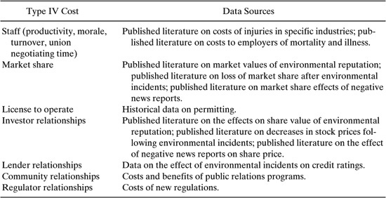
Major categories of internal intangible costs are listed in Table 12.7-1, along with sources of data relevant to estimating these costs. These data sources are described at length in the AIChE CWRT’s Total Cost Accounting methodology.
Brief definitions of each of these cost categories are provided below:
Staff (productivity, morale, turnover, union negotiating time): Poor environmental performance, particularly as reflected in workplace conditions, may lead to increased rates of illness, lower productivity, and more staff turnover.
Market share: Limited anecdotal evidence exists relating negative environmental incidents to loss in market share; other evidence points to the positive influence of “green” handbooks and other environmental ratings.
License to operate: This is not the direct costs associated with obtaining legally required permits; rather, these are costs associated with issues such as delays in receiving permits.
Investor relationships: Relationships with investors can be, at least in part, reflected in stock price.
Lender relationships: Relationships with lenders can be, at least in part, reflected in bond ratings.
Community and regulator relationships: Relationships with regulators and the community are related to license to operate.
Table 12.7-1 Sources of Data on Internal Intangible Costs (AIChE CWRT, 2000).
It is beyond the scope of this chapter to describe the methodologies for estimating all of these costs. Developing cost estimates is made difficult by the variability and uncertainty in much of the data. As an example of this variability and uncertainty, consider the problem of estimating the response of stock prices to environmental reputation. Of the literature reviewed by the AIChE CWRT(2000), some found positive associations between a positive environmental reputation and higher stock prices. Other studies found relationships between negative environmental news or performance and lower stock prices. These studies used widely ranging measures of environmental performance, from emissions reported through the Toxic Release Inventory, to the number of oil spills and whether companies sign on to a set of corporate environmental principles. Thus, it is difficult to design a cost estimation methodology that can employ this broad range of data. Further complicating the situation is the fact that some studies found little to no relationship between stock price and environmental performance.
Nevertheless, these internal intangible costs are widely regarded as real, albeit extremely difficult to quantify.
12.8 External Intangible Costs
External intangible costs are costs borne broadly by communities due to emissions, wastes, resource depletion, and habitat destruction. Examples of these external impacts, which are sometimes referred to as externalities, along with sources of data that can be used to estimate their costs, are listed in Table 12.8-1.
It is beyond the scope of this chapter to describe the methodologies for estimating all of these costs. Instead, since the procedures for estimating the costs in each of the categories have similar features, our focus will be on the procedures. The procedures will be illustrated by considering the cost categories of air pollutant discharges.
Table 12.8-1 Sources of Data on External Intangible Costs (AIChE CWRT, 2000).
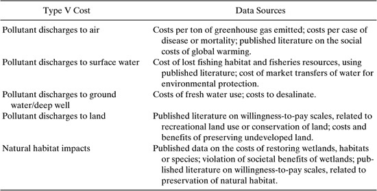
A number of studies have recently appeared attempting to determine actual health-related costs associated with air pollutants, especially ozone and particulate matter. These studies attempt to quantify direct health costs and lost work time associated with air pollutant morbidity and attempt to account for air pollutant mortality by valuing lost earning power and other factors. Typically, when such estimates are done for large urban areas such as Los Angeles and Houston, the costs associated with concentrations of ozone and particulate matter in excess of National Ambient Air Quality Standards are billions of dollars per year. Attributing these externalities to individual emission sources is possible, but would be region-specific and has rarely been done. In contrast, most valuations of externalities rely on surveys that assess the public’s willingness to pay for avoidance of the impacts. The results of willingness-to-pay surveys and other measures of external costs vary widely. The AIChE CWRT (2000), for example, quotes values of external costs ranging from $0.22 to $19 per ton of CO emissions. Particulate matter externalities range from $600 to $26,000 per ton. Similar ranges are reported for Hg, sulfur dioxide, oxides of nitrogen, and a variety of hazardous air pollutants.
References
American Institute of Chemical Engineers Center for Waste Reduction Technologies (AIChE CWRT), “Total Cost Assessment Methodology,” AIChE, New York (ISBN 0-8169-0807-9), 2000.
Hall, J.V., Winer, A.M., Kleinman, M.T., Lurmann, F.W., Brajer, V., and Colome, S.D. (1992), “Valuing the health benefits of clean air,”Science, 255, 812–817.
Heller, M., Shields, P.D., and Beloff, B. (1995) “Environmental Accounting Case Study: Amoco Yorktown Refinery,” Green Ledgers: Case Studies in Corporate Environmental Accounting, D. Ditz, J. Ranganathan, and D. Banks, eds., World Resources Institute (ISBN 1-56973-032-6), Washington, D.C.
Kennedy, M., Total Cost Assessment for Environmental Engineers and Managers, John Wiley & Sons, New York, 1997.
Lurmann, F.W., Hall, J.V., Kleinman, M., Chinkin, L.R., Brajer, V., Meacher, D., Mummery, F., Arndt, R.L., Funk, T.H., Alcorn, S.H., and Kumar, N., “Assessment of the Health Benefits of Improving Air Quality in Houston, Texas,” Final report by Sonoma Technologies to the City of Houston (STI-998460-1875-FR), November, 1999.
Schultz, M.A., “A Hierarchical Decision Procedure for the Conceptual Design of Pollution Prevention Alternatives for Chemical Processes,” Ph.D. Thesis, University of Massachusetts, 1998.
Shields, P., Heller, M., Kite, D., and Beloff, B. (1995) “Environmental Accounting Case Study: DuPont,” Green Ledgers: Case Studies in Corporate Environmental Accounting, D. Ditz, J. Ranganathan, and D. Banks, eds., World Resources Institute (ISBN 1-56973-032-6), Washington, D.C.
United States Congress, Office of Technology Assessment (OTA), “Industry, Technology and the Environment: Competitive Challenges and Business Opportunities,” OTA-ITE-586 (Washington, D.C.: US Government Printing Office, January 1994).
United States Environmental Protection Agency (US EPA), “Pollution Prevention Benefits Manual,” Office of Policy Planning and Evaluation and Office of Solid Waste, 1989.
United States Environmental Protection Agency (US EPA), “A Primer for Financial Analysis of Pollution Prevention Projects,” EPA 600R-93-059, April 1993.
United States Environmental Protection Agency (US EPA), “Valuing Potential Environ-mental Liabilities for Managerial Decision-Making: A Review of Available Techniques,” EPA 742R-96-003, December, 1996.
United States Environmental Protection Agency (US EPA), “An Introduction to Environmental Accounting as a Business Management Tool: Key Concepts and Terms,” EPA 742-R-95-001, June, 1995.
United States Environmental Protection Agency (US EPA), “Searching for the Profit in Pollution Prevention: Case Studies in the Corporate Evaluation of Environmental Opportunities,” EPA 742-R-98-005, April 1998.
Valle-Riestra, J. F., Project Evaluation in the Chemical Process Industries, McGraw-Hill, New York, 1983.
Problems
1. A preliminary process design for a process to produce cyclohexanone ($0.73/lb) and cyclohexanol ($0.83/lb) from cyclohexane ($0.166/lb) and oxygen (from air) results in the following estimates of raw material requirements and waste generation (see Chapter 8):
Raw Materials per mole of cyclohexanone/cyclohexanol
Avg. Molecular weight (MW=99)
1.1 mole cyclohexane (MW=84)
2 moles oxygen (derived from air—no material acquisition cost)
Wastes generated per pound of product
0.060 pound of organics in the gaseous effluent to be treated
0.2 pound of organic aqueous wastes to sent to water treatment
Provide a preliminary estimate of waste treatment costs and compare these to raw material costs per pound of product (Calculate the organic loading in the liquid waste and the total quantity of air to be treated by mass balance).
2. Select a process documented in the AP-42 documents at www.epa.gov/ttn/chief and estimate the costs of waste treatment per pound of product.
3. A chemical manufacturing facility buys raw material for $0.60 per pound and produces 90 million pounds per year of product, which is sold for $0.75 per pound. The process is typically run at 90% selectivity and the raw material that is not converted into product is disposed of at a cost of $0.80 per pound (by incineration). A process improvement allows the process to be run at 98% selectivity, allowing the facility to produce 98 million pounds per year of product. What is the net revenue of the facility (product – sales raw material – costs waste disposal costs) before and after the change? How much of the increased net revenue is due to increased sales of product and how much is due to decreased waste disposal costs?
4. Lurmann, et al. (1999) have estimated the costs associated with ozone and fine particulate matter concentrations above the National Ambient Air Quality Standards (NAAQSs) in Houston. They estimated that the economic impacts of early mortality and morbidity associated with elevated fine particulate matter concentrations (above the NAAQS) are approximately $3 billion/year. Hall, et al. (1992) performed a similar assessment for Los Angeles. In the Houston study, Lurmann, et al examined the exposures and health costs associated with a variety of emission scenarios. One set of calculations demonstrated that a decrease of approximately 300 tons/day of fine particulate matter emissions resulted in a 7 million person-day decrease in exposure to particulate matter concentrations above the proposed NAAQS for fine particulate matter, 17 fewer early deaths per year, and 24 fewer cases of chronic bronchitis per year. Using estimated costs of $300,000 per case of chronic bronchitis and $6,000,000 per early death, estimate the social cost per ton of fine particulate matter emitted. How does this compare to the range of values quoted by the AIChE CWRT? Review the procedures for estimating costs (see Hall, et al., 1992) and comment on the uncertainties associated with the methodology.
5. Browse the website of the World Business Council for Sustainable Development (www.wbcsd.ch) and identify a case study of a company improving business performance through eco-efficiency. Write a one page summary of the case study.