
Chapter 5
Evaluating Environmental Fate: Approaches Based on Chemical Structure
5.1 Introduction
A new chemical is to be manufactured. Will its manufacture or use pose significant environmental or human health risks? If there are risks, what are the exposure pathways? Will the chemical degrade if it is released into the environment or will it persist? If the chemical degrades, will the degradation products pose a risk to the environment?
The challenges involved in answering these questions are formidable. Over 9,000 chemicals are produced commercially and every year, a thousand or more new chemicals are developed. For any chemical in use, there are a number of potential risks to human health and the environment. In general, it will not be possible to rigorously and precisely evaluate all possible environmental impacts. Nevertheless, a preliminary screening of the potential environmental impacts of chemicals is necessary and is possible. Preliminary risk screenings allow businesses, government agencies, and the public to identify problem chemicals and to identify potential risk reduction opportunities. The challenge is to perform these preliminary risk screenings with a limited amount of information.
This chapter presents qualitative and quantitative methods for estimating environmental risks when the only information available is a chemical structure. Many of these methods have been developed by the US Environmental Protection Agency (US EPA) and its contractors. The methods are routinely used in evaluating premanufacture notices submitted under the Toxic Substances Control Act (TSCA). Under the provisions of TSCA, before a new chemical can be manufactured in the United States, a premanufacture notice (PMN) must be submitted to the US EPA. The PMN specifies the chemical to be manufactured, the quantity to be manufactured, and any known environmental impacts including potential releases from the manufacturing site. Based on these limited data, the US EPA must assess whether the manufacture or use of the proposed chemical may pose an unreasonable risk to human or ecological health. To accomplish that assessment, a set of tools has been developed that relate chemical structure to potential environmental risks.
Figure 5.1-1 provides a qualitative summary of the processes that determine environmental risks. Table 5.1-1 identifies the chemical and physical properties that will influence each of the processes that determine environmental exposure and hazard. The table makes clear that a wide range of properties need to be estimated to perform a screening level assessment of environmental risks.
Figure 5.1-1 The chemical and physical properties that will influence each of the processes that determine environmental exposure and hazard.

Table 5.1-1 Chemical Properties Needed to Perform Environment Risk Screenings.
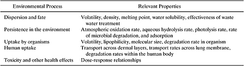
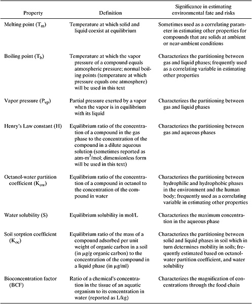
The first group of properties that must be estimated in an assessment of environmental risk are the basic physical and chemical properties that describe a chemical’s partitioning between solid, liquid, and gas phases. These include melting point, boiling point, vapor pressure, and water solubility. Additional molecular properties, related to phase partitioning, that are frequently used in assessing the environmental fate of chemicals include octanol-water partition coefficient, soil sorption coefficients, Henry’s Law constants and bioconcentration factors. (Each of these properties is defined in Section 5.2). Once the basic physical and chemical properties are defined, a series of properties that influence the fate of chemicals in the environment are estimated. These include estimates of the rates at which chemicals will react in the atmosphere, the rates of reaction in aqueous environments and the rate at which the compounds will be metabolized by organisms. If environmental concentrations can be estimated based on release rates and environmental fate properties, then human exposures to the chemicals can be estimated. Finally, if exposures and hazards are known, then risks to humans and the environment can be estimated.
The remainder of this chapter describes estimation tools for the properties outlined above. Section 5.2 describes estimation tools for physical and chemical properties. Section 5.3 describes how properties that influence environmental fate are estimated. Methods for estimating hazards to ecosystems are discussed in Section 5.4, and Section 5.5 presents simple models that can be used to characterize the environmental partitioning of chemicals. Finally, Section 5.6 describes how chemical property data can be used to classify the risks associated with chemicals.
5.2 Chemical and Physical Property Estimation
Although many chemical and physical properties can influence the way in which a chemical partitions in the environment, most screening-level evaluations focus on only a small number of properties. These properties describe the partitioning of chemicals between solid, liquid and gaseous phases and include melting point, boiling point, and vapor pressure. Additional molecular properties, related to phase partitioning, that are frequently used in assessing the environmental fate of chemicals include Henry’s law constants, octanol-water partition coefficient, water solubility, soil sorption coefficients and bioconcentration factors. Table 5.2-1 defines each of these properties and describes the significance of the property in estimating environmental fate.
Table 5.2-1 Properties that Influence Environmental Phase Partitioning.
This section describes how each of these properties can be estimated based on the structure of the chemical. The review of estimation methods will not be comprehensive. Rather, the focus is on presenting commonly used methods that can produce property estimates based only on the chemical structure of the target compound. More complete presentations are available in texts on environmental property estimation (e.g., Lyman, et al., 1990). More complete compilations of data are available from Howard (1997), Mackay, et al. (1992), Reinhard and Drefahl (1999), and the sources listed in Appendix F.
The methods described in this section generally assume that a molecule is composed of a collection of functional groups or molecular fragments and that each fragment contributes in a well-defined manner to the properties of the molecule. These methods are generally described as group contribution methods, structure activity relationships (SARs) or quantitative structure activity relationships (QSARs).
5.2.1 Boiling Point and Melting Point
As a first example of a structure activity relationship, consider the estimation of boiling point (at one atmosphere pressure). Boiling point is influenced by molecular weight and intermolecular attractions. It can be estimated using a relatively simple group contribution method, developed by Joback and Reid (1987) and modified by Stein and Brown (1994), that relates the boiling point to the number and type of functional groups present in the molecule.
![]()
where Tb is the normal boiling point (at one atmosphere pressure) in degrees Kelvin, ni is the number of groups of type i in the molecule, gi is the contribution of each group to the boiling point, and the summation is taken over all groups. The boiling point predicted by Equation 5-1 is corrected using one of the following equations:
![]()
![]()
Structural groups and group contributions (gi) for boiling point estimation are listed in Table 5.2-2. When tested against a set of more than 4000 organic compounds, this method yielded an average error of 3.2% (Stein and Brown, 1994).
Table 5.2-2 Structural Groups and Group Contributions for Boiling Point Estimation (Stein and Brown, 1994).

Although Equations 5-1 to 5-3 are not the only method or even the most accurate method for estimating boiling point (for a more complete discussion, see Reid, et al., 1987), the approach does illustrate the basic principles of a group contribution method. Each functional group in a molecule is assumed to make a well-defined contribution (in this case, gi) to the property. The group contributions may be simply added together, as in Equation 5-1, or a more complex mathematical form may be used. The application of the method is illustrated in Example 5.2-1.
Example 5.2-1
Estimate the normal boiling point for ethanol, toluene, and acetaldehyde.
Solution: Ethanol has the molecular structure CH3–CH2 –OH. Referring to the groups in Table 5.2-2, this structure can be represented by one –CH3 group, one –CH2 group and one –OH group. The uncorrected normal boiling point, from Equation 5-1, is given by:
Tb(K) = 198.2 + 21.98 + 24.22 + 88.46 = 332.9 K
The corrected value is:
Tb(corrected) = Tb – 94.84 + 0.5577Tb – 0.0007705(Tb)2 = 338.3 K
The actual boiling point is 351 K, so the predicted value is in error by –3.6 %
Toluene has the molecular structure CH3–C6H5. Referring to the groups in Table 5.2-2, this structure can be represented by one –CH3 group, one –aa C– group (a substituted carbon bound to two aromatic carbons) and five –aa CH– groups. The uncorrected normal boiling point, from Equation 5-1, is given by:
Tb(K) = 198.2 + 21.98 + 30.76 + 5(28.53) = 393.6 K
The corrected value is:
Tb(corrected) = Tb – 94.84 + 0.5577Tb – 0.0007705(Tb)2 = 398.9 K
The actual boiling point is 384 K, so the predicted value is in error by +3.9%
Acetaldehyde has the molecular structure CH3 –CH=O. Referring to the groups in Table 5.2-2, this structure can be represented by one –CH3 group and one –CHO group. The uncorrected normal boiling point, from Equation 5-1, is given by:
Tb(K) = 198.2 + 21.98 + 83.38 = 303.6 K
The corrected value is:
Tb (corrected) = Tb – 94.84 + 0.5577Tb – 0.0007705(Tb)2 = 307.0 K
The actual boiling point is 294 K, so the predicted value is in error by +4.2%
While group contribution methods can produce accurate estimates of chemical and physical properties, it is important to recognize their limitations. Group contribution equations are empirical. They are designed to accurately reflect a particular set of property data. If a group contribution method is used to estimate the properties of molecules that have structures significantly different from those used in the original data set, substantial errors can result. Consider, for example, what might happen if a group contribution method, originally developed with data on alcohols, was used to estimate the properties of glycols. Since glycols have two hydroxyl groups per molecule, they can form chains of molecules (n-mers) held together by hydrogen bonding forces. In contrast, alcohols, with only one hydroxyl group per molecule, can only form dimers in solution. A group contribution method for boiling point, developed with data on alcohols, would likely underpredict the boiling point of glycols (see Example 5.2-2).
Example 5.2-2
Estimate the normal boiling point for ethylene glycol.
Solution: Ethylene glycol has the molecular structure HO–CH2–CH2–OH. Referring to the groups in Table 5.2-2, this structure can be represented by two–CH2 groups and two –OH groups. The uncorrected normal boiling point, from Equation 5-1, is given by:
Tb(K) = 198.2 + 2(24.22) + 2(88.46) + 424 K
The corrected value is:
Tb(corrected) = Tb – 94.84 – 0.5577Tb – 0.00077051Tb22 = 427 K
The actual boiling point is 470 K, so the predicted value is in error by –9%.
As shown in Example 5.2-1, the estimation of boiling point, using Equations 5-1 to 5-3, is relatively straightforward. Boiling points, in turn, can be used to estimate a variety of other properties. One property, which is occasionally used in estimating the phase partitioning of solids, is melting point. Melting point is sometimes expressed as a simple fraction of boiling point (Lyman, 1985):
![]()
5.2.2 Vapor Pressure
The vapor pressure of a chemical plays a significant role in its environmental partitioning. High vapor pressure materials will generally have higher atmospheric concentrations than lower vapor pressure materials, and therefore, have the potential to be transported over long distances as gases or inhaled as gases. The temperature dependence of vapor pressure also plays a role in environmental transport and partitioning. If a chemical’s vapor pressure varies significantly between daytime and nighttime conditions, strong daily cycling of the chemical between environmental media can be expected, assuming no degradation or soil adsorption. Finally, vapor pressures are used in a variety of ways in estimations of exposure and environmental risk. Therefore, reliable estimates of vapor pressure, over a range of temperatures, will be important in screening chemicals for environmental risk.
A number of approaches are available for estimating vapor pressures. Some approaches are based on critical temperatures and pressures; others rely on heats of vaporization (Lyman, et al., 1990). Still other methods use estimates of vapor pressure at a reference temperature (such as the boiling point) to estimate vapor pressure. The methods based on boiling point and heat of vaporization will be the focus of this section—not because they are necessarily more accurate than the other methods, but rather, because they are conveniently estimated from chemical structure.
One method for estimating vapor pressure from boiling point and heat of vaporization uses the mathematical form associated with the Antoine equation:
![]()
Where Pvp is the vapor pressure, A and C are empirical constants, B is a parameter that is related to the heat of vaporization and T is absolute temperature. A derivation of this equation based on thermodynamic concepts is available in Lyman, et al. (1990) and in most thermodynamic textbooks.
Note that if we apply Equation 5-5 at the boiling point and define the units of vapor pressure as atmospheres, then:
![]()
Equation 5-6 can be used to express the parameter B in terms of A, C and Tb. Lyman, et al. (1990) provide a derivation of the following equation,
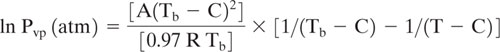
where R is the gas constant (1.987 l-atm °K−1 mol−1). Empirical correlations are available for estimating the parameters A and C from boiling point:
![]()
![]()
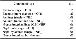
Equations 5-7 through 5-9 allow vapor pressure to be estimated, as a function of temperature, based only on the boiling point and the parameter KF. Values of KF are given in Tables 5.2-3 and 5.2-4. For any compound not given in the tables, assume KF = 1.06.
Equations 5-7 through 5-9 work well in estimating vapor pressures that range from 10-2 to one atmosphere, yielding average errors of 2.7%. The performance deteriorates at lower pressures, with average errors of 86% for vapor pressures ranging from 10−6 to 10−2 atmosphere (Lyman, et al., 1990).
For solids, a slightly different form is generally used:
![]()
where P is the vapor pressure in atmospheres, Tb is the normal boiling point (K), T is the temperature at which the vapor pressure is to be evaluated (K), and Tm is the melting point (K).
Care must be taken in defining the units for Equations 5-7 through 5-10. Example 5.2-3 illustrates the proper use of units.
Table 5.2-3 Factors (KF) Used in estimating Boiling Point (Lyman, et al., 1990)
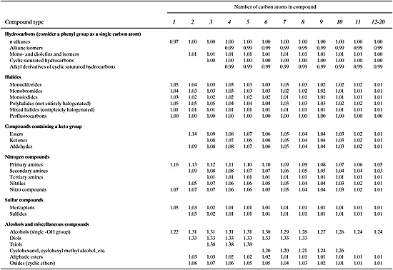
Table 5.2-4 Factors (KF) Used in Estimating Boiling Points for Aromatics (Lyman, et al., 1990).
Example 5.2-3
Estimate the vapor pressure at 298 K for toluene (a liquid) and naphthalene (a solid).
Solution: Toluene has the molecular structure CH3 –C6H5 and in Example 5.2-1, its boiling point was estimated to be 399 K. The experimental value for the boiling point is 384 K. We will estimate the vapor pressure using both the predicted and the experimental value for boiling point. Using the predicted value of 399 K:
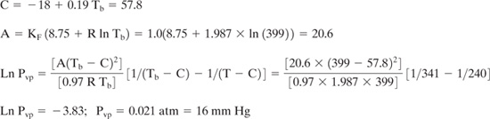
Repeating the calculation for the experimental boiling point leads to a vapor pressure estimate of 19 mm Hg.
Naphthalene has the formula C10H8 and is a solid with a melting point of 81°C. The boiling point can be estimated from the methods described earlier in this section. The uncorrected group contribution estimate is:
Tb = 198.2 + 2(45.46) + 8(28.53) = 517 K
The corrected value is: Tb = 505 K
Applying Equation 5-10:
ln P = –(4.4 ln Tb)[1.803(Tb/T–1) –0.803 ln(Tb/T)] –6.8(Tm/T –1) |
ln P = –(4.4+ln 505)[1.803 (505/298 –1) –0.803 ln(505/298)] –6.8(354/298 –1) |
P = 4.4 ×10⁻⁵ atm = 0.03 mm Hg |
5.2.3 Octanol-Water Partition Coefficient
While melting points, boiling points, and vapor pressures are familiar properties used in many applications, properties such as the octanol-water partition coefficient are more specialized parameters used in environmental fate modeling. The octanol-water partition coefficient is used to characterize the partitioning of a molecule between largely aqueous phases, such as rivers and lakes, and largely hydrophobic phases, such as the organic fraction of sediments suspended in water bodies. Because the octanol water partition coefficient (Kow) characterizes partitioning between aqueous and organic, lipid-like phases, it is used to estimate a variety of toxicological, and environmental fate parameters. Therefore, accurate estimates of Kow are critical to successful estimates of other environmental properties.
One specific and simple use of the octanol-water partition coefficient is as a gauge for the potential for bioaccumulation. If a chemical tends to partition into the organic phase (is lipophilic), then the chemical can be stored in fatty tissue of fish and will bioaccumulate in animals that consume the fish. Table 5.2-5 describes the approximate relationship between Kow and bioaccumulation.
Group contribution methods (structure activity relationships) have been developed for octanol-water partition coefficients (Meylan and Howard, 1995), and they have a form very similar to the form used for boiling point.
![]() (Eq. 5-11)
(Eq. 5-11)
where log Kow is the base 10 logarithm of the ratio of the chemical’s mass fraction in octanol to the chemical’s concentration in water, ni is the number of groups of type i in the molecule, fi is the contribution of each group to the partition coefficient, and the summation is taken over all groups. Structural groups and group contributions (fi) for estimating octanol-water partition coefficients are listed in Table 5.2-6.
Just as was done for boiling point, corrections are introduced to the preliminary estimate. In this case, corrections account for the unusual behavior of selected functional groups. The equation for estimating the corrected value of Kow is:
![]()
where nj is the number of groups of type j in the molecule, cj is the correction factor for each group, and the summation is taken over all groups that have correction factors. Structural groups and correction factors (cj) are listed in Table 5.2-7. The method yields a mean error of 0.31 log units (Meylan and Howard, 1995).
On first inspection, the correction factors listed in Table 5.2-7 may seem a bit baffling and arbitrary; however, more careful analysis reveals the rationale behind the corrections. For example, many of the corrections account for electronic interactions between multiple substituents on aromatic rings (e.g., all of the orthocorrections in Table 5.2-7). Recall from organic chemistry that substituents on aromatic rings can be electron donating or electron withdrawing and that these electronic effects are different at ortho-, meta- and para- positions. Thus, if there are two or more substituents on an aromatic ring, the substituents will interact with one another through their electronic effects on the ring. The corrections in the table account for this effect. Other corrections in Table 5.2-7 account for other types of interactions between groups and the presence of ring structures. A final type of correction in the table accounts for the presence of multiple hydrogen bonding groups in a molecule. Molecules with one hydrogen bonding group can form dimers, while molecules with more than one hydrogen bonding group can form n-mers. The potential formation of polymer-like chains held together by hydrogen bonds can dramatically influence chemical and physical properties, necessitating correction factors for molecules containing multiple hydrogen bonding groups.
Table 5.2-5 Classification Criteria for Bioaccumulation.
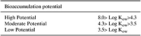
Table 5.2-6 Structural Groups and Group Contributions for Estimating Octanol-Water Partition Coefficients (Meylan and Howard, 1995).
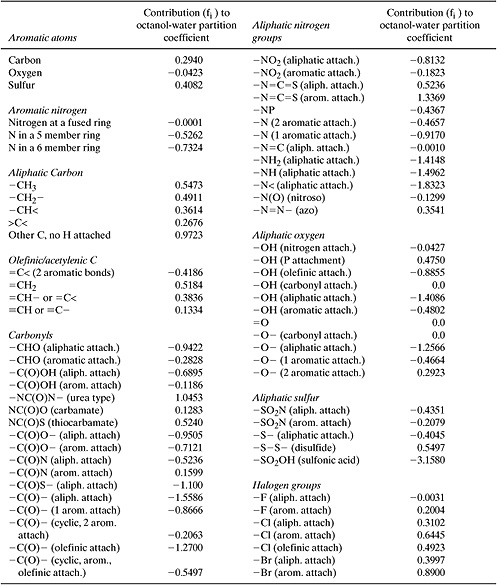
Table 5.2-7 Correction Factors for Estimating Octanol-Water Partition Coefficients (Meylan and Howard, 1995).

While a list of correction factors could potentially be endless, in practice, only a few types of corrections are normally accounted for. Ring correction factors, factors accounting for multiple hydrogen bonding groups, and corrections for substitution positions are among the most common. Example 5.2-4 illustrates the use of the group contribution method and the application of correction factors.
Example 5.2-4
Estimate the octanol-water partition coefficient for 1,1 dichloroethylene and the structure shown below (a herbicide).
Figure 5.2-1 Structure of herbicide.
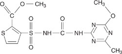
Solution: 1,1-Dichloroethylene has the molecular structure CH2=CCl2. Referring to the groups in Table 5.2-6, this structure can be represented by one =CH2 group, one =CH or =C< group and two –Cl(olefinic attachment) groups. The uncorrected value of Kow from Equation 5-4 is given by:
log Kow |
= 0.229 + 0.5184 + 0.3836 + 2(0.4923) = 2.11 |
Kow |
= 130 |
Dichloroethlene does not contain any groups that have correction terms. The experiment value for log Kow is 2.13, so the predicted value of log Kow is in error by 3.3%.
The herbicide can be represented by three –CH3 groups, one –NH– (aliphatic attachment), 7 aromatic carbons, 3 aromatic nitrgens, one –O– (one aromatic atachment) group, one –N(one aromatic atachment) group, one aromatic sulfur group, one –C(=O)O (ester, aromatic attachment) group, one –SO2 N(aromatic attachment) group and one –NC(=O)N– (urea type carbonyl) group. Note that the –NC(=O)N– is listed as a carbonyl group in Table 5.2-7 and accounts only for the carbonyl(C=O), not the nitrogens. The uncorrected value of Kow from Equation 5-4 is given by:
log Kow = | 0.229 + 3(0.5473) – 1.4962 + 7(0.2940) + 3(0.7324) – 0.4664 – 0.9170 + |
| 0.4082 –0.7121– 0.2079 + 1.0453 = –0.614 |
The herbicide contains several groups that require correction factors. There is one triazine ring correction (0.8856), one correction for an amino-type triazine (0.8566), one correction for an alkoxy ortho to two aromatic nitrogens (0.8955) and one correction for a –NC(=O)NS on a triazine (–0.7500). The total of these correction facors is 1.887, leading to
log Kow = 1.273
The octanol-water partition coefficient for this compound is strongly pH-dependent, but this estimation method leads to reasonable estimates for slightly basic solutions.
5.2.4 Bioconcentration Factor
One of the primary reasons for estimating the octanol-water partition coefficient is to assess the partitioning of a chemical between aqueous and lipid phases in living organisms. This partitioning is normally expressed as a bioconcentration factor (BCF). The BCF is defined as the ratio of a chemical’s concentration in the tissue of an aquatic organism to its concentration in water (in L/kg). This parameter is called a bioconcentration factor because high values of BCF indicate that a living organism will tend to extract a material from an aqueous phase, such as ingested water or blood, and concentrate it in lipid tissues (e.g., fats). Thus, high values of BCF can be cause for concern. For example, a compound with a high bioconcentration factor may tend to accumulate in fish, resulting in a health hazard if the fish is eaten.
As shown in Table 5.2-8, BCF values can be used to gauge bioaccumulation potential, just as octanol-water partition coefficients were (Table 5.2-5).
Veith and Kosian (1983) propose this correlation between octanol-water partition coefficients and BCF:
Table 5.2-8 Classification Criteria for Bioaccumulation.

More recently, correction factors have been introduced into this correlation, in a manner analogous to the estimation methods for Kow. For non-ionic compounds, Meylan, et al. (1997), propose:
![]()
where jj is the correction factor for each group, and the summation is taken over all groups that have correction factors. The correction factors are listed in Table 5.2-9. Mean errors of approximately 0.5 log units can be expected with this method.
Note that there are fewer correction factors in Table 5.2-9 than in Table 5.2-7. This is not because BCF is more straightforward to estimate than Kow. If anything, BCF is more difficult to reliably estimate than Kow because of the variability in lipid tissues. The reason why Table 5.2-9 is relatively sparse is because experimental values, on which the correction factors are based, are considerably scarcer for BCF than for Kow. Therefore, estimates of BCF for structurally complex compounds that typically require correction factors may have considerable uncertainty.
Example 5.2-5
Estimate the bioconcentration factor for 2,2,4 trimethyl-1,3 pentanediol, and 2,4’,5 trichlorobiphenyl.
Solution: 2,2,4 trimethyl-1,3 pentanediol has the structure HO–CH2–(C)(CH3)2–CH(OH)–(CH)(CH3)–CH3. Before estimating BCF, it is first necessary to estimate Kow. Referring to the groups in Table 5.2-6, the structure can be represented by four –CH3 groups, one –CH2– group, one >C< group, two CH< groups and two –OH groups (aliphatic attachment). The uncorrected value of Kow from Equation 5-4 is given by:
log Kow = 0.229 + 4(0.5473) + 0.4911 + 0.2676 + 2(0.3614) + 2(–1.4086) = 1.08
Kow = 12.1
2,2,4 trimethyl-1,3 pentanediol requires a correction for molecules containing two or more aliphatic –OH(0.4064). The corrected value for log Kow is 1.49. The experimental value for log Kow is 1.24. Using the corrected calculated value of log Kow and Equation 5-13 (Equation 5-14 does not apply because none of the correction factors in Table 5.2-9 are appropriate), proceed to calculate BCF for 2,2,4 trimethyl-1,3 pentanediol.
log BCF = 0.79(1.49) – 0.49 = 0.7771
BCF = 5.99
Referring to Table 5.2-8, we see that because the BCF of 2,2,4 trimethyl-1,3 pentanediol is less than 250, it has low potential for bioaccumulation.
2,4’,5 trichlorobiphenyl can be represented by 12 aromatic carbons and 3 –Cl (aromatic attachment) groups. The uncorrected value of Kow from Equation 5-4 is given by:
log Kow = 0.229 + 12(0.2940) + 3(.6445) = 5.69
Table 5.2-9 Correction Factors for BCF of Non-Ionic Compounds (Meylan and Howard, 1997).
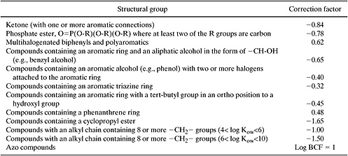
No corrections are required. The experimental value for log Kow is 5.81. Using this uncorrected calculated value of log Kow and Equation 5-14, proceed to calculate BCF for 2,4’,5 trichlorobiphenyl. With the correction factor from Table 5.2-9 for multihalogenated biphenyls and polyaromatics (0.62), Equation 5-14 becomes:
log BCF = 0.77(5.59) – 0.70 + 0.62 = 4.30
BCF=20000
Referring to Table 5.2-8, it is evident that 2,4’,5 trichlorobiphenyl has a very high potential for bioaccumulation.
5.2.5 Water Solubility
In assessing environmental transport and partitioning, it is often necessary to predict maximum, or saturation, concentrations. In the gas phase, this is done by estimating vapor pressure. In aqueous phases, saturation concentrations are estimated using water solubilities.
Water solubility can be estimated in many ways. Activity coefficients, solubility parameters, and other chemical and structural properties can be used as a basis for estimating water solubility. For environmental applications, however, water solubility is most often estimated based on octanol-water partition coefficients. This is not because Kow is the most accurate or reliable parameter for estimating water solubility. Rather, it is a matter of convenience. Kow is used to estimate a wide variety of parameters in evaluating environmental fate and risk. Therefore, Kow is generally available in environmental assessments, while properties such as activity coefficients are not frequently calculated in environmental screening studies. Table 5.2-10 classifies the numerical values for solubility (S) into general solubility categories.
Table 5.2-10 Classification Criteria for Water Solubility.

Meylan, et al. (1996) have used Kow, along with correction factors, to estimate water solubilities. Their correlations are:
![]()
![]()
![]()
where S is the water solubility in mol/L; Kow is the octanol-water partition coefficient, Tm is the melting point in °C, MW is the molecular weight, and hj is the correction factor for each group, and the summation is taken over all groups that have correction factors. Note that the correction factors are different for each equation. They are listed in Table 5.2-11. Mean errors are in the range of 0.3 to 0.4 log units.
Any of the three equations can be used, but generally, if more information is available for the correlation (Equations 5-16 or 5-17), the estimate is more accurate.
Example 5.2-6
Estimate the water solubility of 2-hexanol and diphenyl ether.
Solution: 2-hexanol has the molecular structure CH3–(CH–OH)–C4 H9. Before estimating water solubility, we must estimate Kow. Referring to the groups in Table 5.2-6, this structure can be represented by two –CH3 –groups, three –CH2 –groups, one –CH– group and one –OH (aliphatic attachment) group. The uncorrected value of Kow from Equation 5-11 is given by:
log Kow = 0.229 + 2(0.5473) + 3(0.4911) + 0.3614 – 1.4086 = 1.75
2-hexanol does not contain any groups that have correction terms. The experimental value for log Kow is 1.76, so the predicted value of Kow is in error by y –0.6 %.
The water solubility can be estimated from Equation 5-16 with a correction term for one aliphatic –OH group.
Log S = 0.796 – 0.854(log Kow) – 0.00728(MW) + ∑hj
Log S = 0.796 –0.854(1.75) – 0.00728(102.2) + 0.510 = –0.932
S = 0.12 mol/L
Diphenyl ether has the molecular structure C6H5–O–C6H5. Before estimating water solubility, we must estimate Kow. Referring to the groups in Table 5.2-6, this structure can be represented by twelve aromatic carbons and one –O– group (two aromatic attachments) group. The uncorrected value of Kow from Equation 5-11 is given by:
log Kow = 0.229 + 12(0.2940) + 0.2923 = 4.05
Table 5.2-11 Correction Factors for Estimating Water Solubility (Meylan, et al., 1996).

Diphenyl ether does not contain any groups that have correction terms. The experimental value for log Kow is 4.21, so the predicted value of log Kow is in error by –3.8 %.
The water solubility can be estimated from Equation 5-16. There are no correction terms that apply.
Log S = 0.796 – 0.854(log Kow) – 0.00728(MW) + ∑hj
Log S = 0.796–0.854(4.05) – 0.00728)(170.2) + 0.0 = –3.90
S = 1.2 × 10⁻⁴ mol/L
5.2.6 Henry’s Law Constant
The Henry’s Law constant, as commonly used in describing environmental fate, is the ratio of a compound’s concentration in air to its concentration in water, at equilibrium. In other words, it shows a compound’s affinity for air over water.
Therefore, compounds with high values of Henry’s Law constant (H) tend to partition into the air, while compounds with low values of H tend to partition into the water. H is generally expressed either as a dimensionless ratio of concentrations of the compound (in mol/m3) in the vapor and aqueous phases, or in units of atm-m3/mole. (Table 5.2-12)
A group contribution method can also be used to estimate the value of the Henry’s Law constant. In this case, the group contribution method is structured differently from the previous methods. The structural elements are bonds rather than functional groups. Consider 1-propanol as an example of how a bond approach differs from a functional group approach to structural characterization.
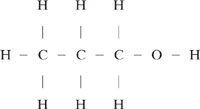
Using the groups from Table 5.2-2, 1-propanol consists of one –CH3 group, two >CH2 groups, and one primary –OH group. Expressed as a collection of bonds, 1-propanol has of 7 C-H bonds, 2 C-C bonds, one C-O bond and one O-H bond.
A preliminary estimate of the Henry’s Law constant is obtained by summing each of the bond contributions. This preliminary estimate is then adjusted by correction factors for selected functional groups (Meylan and Howard, 1991).
![]()
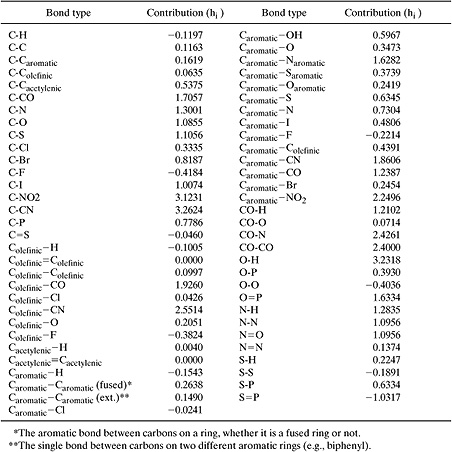
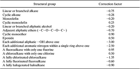
where H is the dimensionless Henry’s Law constant, ni is the number of bonds of type i in the molecule, hi is the bond contribution to the air-water partition coefficient, nj is the number of groups of type j in the molecule, cj is the correction factor for each group, and the summations are taken over all bonds and all groups that have correction factors. Bond contributions (hi) and correction factors (cj) are listed in Tables 5.2-13 and 5.2-14. Mean errors in log units range from 0.06 for alkanes and alkylbenzenes to 0.4 for haloalkenes (Meylan and Howard, 1991).
Table 5.2-12 Classification Criteria for Volatility.
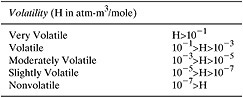
Table 5.2-13 Structural Groups and Group Contributions for Estimating Henry’s Law Constants (Meylan and Howard, 1991).
Example 5.2-7
Estimate the Henry’s Law constant for 1-propanol.
Solution: 1-propanol consists of 7 C-H bonds, 2 C-C bonds, one C-O bond and one O-H bond.
The uncorrected value of log (air to water partition constant) is given by:
–log H = log | (air–water partition coefficient) = |
| 7(–0.1197) + 2(0.1163) + 1.0855 + 3.2318 = 3.7112 |
The correction is for linear or branched alcohols(–0.20) giving a net value of 3.5112 for log H-1. The experimental value is 3.55, an error of –1.1% in the logarithm of the air to water partition constant. Note that this is a dimensionless value (mol/m3 divided by mol/m3). To convert to units of atmospheres-m3/mol, the dimensionless value should be adjusted using the ideal gas law, the gas constant, and the temperature.
Table 5.2-14 Correction Factors for Henry’s Law Constants (Meylan and Howard, 1991).
5.2.7 Soil Sorption Coefficients
Soil-water partitioning is generally described using soil sorption coefficients. The coefficient (Koc) is defined as the ratio of the mass of a compound adsorbed per unit weight of organic carbon in a soil (in μg/g organic carbon) to the concentration of the compound in a liquid aqueous phase (in μg/ml). Values of Koc are categorized in Table 5.2-15.
The property estimation methods just described for water solubility, bioconcentration factor, and Henry’s Law constant used the octanol-water partition coefficient as the primary correlating variable. This was possible because both the properties of interest and the correlating variable were bulk properties.
Table 5.2-15 Classification Criteria for Soil Sorption.

Correlations for soil sorption coefficients, based on octanol-water partition coefficients and water solubility, are also available.
Lyman, et al. (1990) have given the following equations for soil sorption coefficient estimation.
![]()
![]()
These equations, however, are restricted to quite specific classes of compounds. They are limited in their applicability because of the nature of soil sorption. The soil sorption coefficient describes the physical adsorption and chemical absorption of a compound onto a surface. The coefficient therefore depends not only on bulk properties, but also on steric properties that influence the interaction of a molecule with a surface. Meylan, et al. (1992) have proposed a relatively simple correlation for estimating soil sorption coefficients that incorporates both bulk and steric effects through a structural parameter called the molecular connectivity.
![]()
where Koc is the soil sorption coefficient expressed as the ratio of the mass of a compound adsorbed per unit weight of organic carbon in a soil (in μg/g organic carbon) to the concentration of the compound in a liquid phase (in μg/ml);1χ is the first order molecular connectivity index, as described in Appendix B; nj is the number of groups of type j in the molecule; Pj is the correction factor for each group, and the summation is taken over all groups that have correction factors. The correction factors are listed in Table 5.2-16. Mean errors of approximately 0.6 log units can be expected.
Example 5.2-8
Estimate the soil sorption coefficient of 2-hexanol.
Solution: As noted in Example 5.2-6, 2-hexanol has the molecular structure CH3–(CH–OH)–C4H9. Log Kow was estimated to be 1.75 and log S was estimated to be 0.932. Estimating soil sorption coefficients using Equation 5-19 and Equation 5-20:
Log Koc = 0.544 log Kow + 1.377 = 2.329
Log Koc = –0.55 log S + 3.64 = 4.15
Both of these estimates are substantially different from the experimental value of 1.01. Using instead a correlation based on molecular connectivity (Equation 5-21):
Log Koc = 0.531χ + 0.62 + Σ njpj
Where the value of 1x is 3.27 gives an uncorrected value of 2.35. Adding in the correction term for an aliphatic alcohol (–1.519) yields an estimate of 0.83.
Table 5.2-16 Correction Factors for Soil Sorption Coefficients (Meylan and Howard, 1992).
Summary
This section has examined methods for estimating chemical and physical properties that influence phase partitioning in the environment. These methods will serve as the basis for estimation of a broad range of parameters that describe environmental persistence and environmental impacts. Therefore, any errors or uncertainties associated with the estimates described in this section are likely to propagate through the entire environmental assessment.
Section 5.2 Questions For Discussion
1. How would you estimate properties for molecules that contain groups that are not explicitly represented in the group contribution methods (for example, could you estimate the Henry’s Law constant for the herbicide listed in Example 5.2-3?).
2. The methodologies presented in this chapter are only a small selection of the group contribution methods available for these properties. How would you select the most accurate estimation methods?
3. Do the functional forms of the group contribution methods seem appropriate? For example, is it reasonable to assume that a boiling point estimation method should be a simple linear function? Would this approach work equally well for carboxylic acids and dicarboxylic acids? Would it work equally well for alcohols and glycols?
4. Can you rationalize the values of the group contributions? For example, does it make sense that the OH group has a large positive group contribution for boiling point?
5.3 Estimating Environmental Persistence
Section 5.2 described estimation tools for properties that influence the phase partitioning of chemicals in the environment. This section will examine methods for estimating the persistence of chemicals in the atmosphere and in aqueous and sediment environments. These methods are, by necessity, extremely simplified attempts to characterize the complex chemistries that occur in ambient environments. Thus, they should not be viewed as precise tools for estimating environmental lifetimes of chemicals. Rather, they should be viewed as semi-quantitative screening tools for ranking relative persistence.
5.3.1 Estimating Atmospheric Lifetimes
Chemicals emitted to the atmosphere undergo oxidation through a wide range of processes. One of the critical steps in these oxidations, particularly for organic compounds, is the rate of reaction with the hydroxyl radical. Hydroxyl radicals are extremely reactive species and can abstract hydrogen from saturated organics, add to double bonds or add to aromatic rings. Some of these reactions are shown below.
Hydrogen abstraction from propane
Hydroxyl radical addition to propene
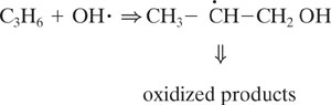
Hydroxyl radical addition to an aromatic ring
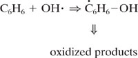
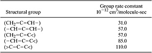
These reactions with hydroxyl radicals are often the first step in a series of reactions that lead to the oxidation of organics in the atmosphere. We do not examine the details of these pathways (the interested reader is referred to Seinfeld and Pandis, 1998); however, the relative rate at which a hydroxyl radical reacts with a compound is a semi-quantitative indicator of how long the compound will persist in the atmosphere. For example, for the three reactions listed above (hydrogen abstraction from propane, addition to propene, and addition to benzene), the rates of reaction are 1.2 × 10⁻¹², 26.0 × 10⁻¹², and 2.0 × 10⁻¹² cm3/molecule-sec., respectively. This indicates that if reaction with a hydroxyl radical is the dominant reaction pathway leading to oxidation in the atmosphere, then the rates of disappearance should be in the ratio 1.2:26:2. As shown in Example 5.3-1, this implies a ratio of atmospheric lifetimes of 106 hours:5 hours:64 hours.
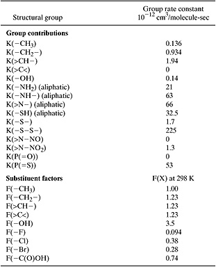
So, one method of assessing atmospheric lifetimes is to estimate rate of reaction with hydroxyl radical. Once again, group contribution methods are a viable approach. The mechanics of the method are similar to those discussed in Section 5.2. A molecule is divided into a collection of functional groups and each group makes a defined contribution to the overall rate of reaction. The method is slightly different from the methods discussed in Section 5.2, however, in that a single compound might have multiple rate parameters. Consider, for example, the reactions of propene. Hydroxyl radical can add to the double bond of propene. To estimate that rate constant, we would note that the olefinic group in propene has the structure (CH2 = CH–), and based on the data in Table 5.3-2, the rate constant for hydroxyl radical addition would be 26.3 × 10⁻¹² cm3/molecule-sec. But hydroxyl radical can also abstract hydrogen from the terminal methyl group. This reaction, however, occurs much more slowly than the addition reaction. The group contribution for abstraction from a terminal methyl group is only 0.136 × 10⁻¹² cm3/molecule-sec (Table 5.3-1). Thus, although propene can react via two pathways, only one is significant.
Identifying and estimating the rates of hydroxyl radical reactions with all of the functional groups in a molecule requires extensive experience. In this chapter, we will limit our estimations to addition reactions for olefins, and abstraction reactions. The group contributions for estimating these rates are listed in Tables 5.3-1 to 5.3-3. As with the property estimations described in Section 5.2, there are correction factors that can be applied to the estimations. These correction factors account for the electron donating and withdrawing characteristics of substituent groups, ring strain energy, and other parameters. A detailed discussion of these correction factors is beyond the scope of this chapter. Examples 5.3-1 through 5.3-3 illustrate how the basic estimations of hydroxyl radical reaction rates and atmospheric half-life are performed and provide simple illustrations of how the correction factors are applied.
Example 5.3-1
Using the rate of reaction of propene with the hydroxyl radical, estimate the atmospheric half-life of propylene.
Solution: The rate of reaction implies a rate of disappearance of propene:
(d[Cpropene]/dt) = k [OH·] [Cpropene]
where [OH·] is the concentration of the hydroxyl radical and [Cpropene] is the concentration of propene.
Assuming that the concentration of hydroxyl radical is at steady state—the pseudosteady-state assumption (see, for example, Fogler, 1995)—leads to the following expression for the concentration of propene:
In ([Cpropene]/[Cpropene]) = - (k [OH·])t
where [C0-propene] is the initial concentration of propene, (k [OH·]) is the rate constant multiplied by the steady state concentration of hydroxyl radicals and t is the time of reaction.
Since ([Cpropene]/[C0-propene])=1/2 when the concentration has reached one half of its original value, the half life is given by:
t1/2 = In (2) / (k[OH·])
Assuming a value of 1.5×10⁶ molecules/cm3 for the concentration of the hydroxyl radical (while 1.5×10⁶ molecules/cm3 is a typical value, summertime concentrations in urban areas can reach 107 molecules/cm3) and a value of 26 10 12 cm3/molecule-sec for k:
t1/2= In (2)/(39×10-6sec-1)
So, the half life for propene in the atmosphere is:
t1/2=5.0 hr
Repeating this calculation for propane and benzene, with reaction rates of 1.2×10⁻¹² and 2.0×10⁻¹² cm3/molecule-sec, leads to atmospheric half lives of 106 and 64 hours, respectively.
Estimate the rate of reaction of octane with the hydroxyl radical.
Solution: Octane has the molecular structure CH3 –(CH2)6 –CH3. Since there are no aromatic, olefinic, or acetyl groups, the primary reaction pathway will be hydrogen atom abstraction. Referring to the groups in Table 5.3-1, this structure can be represented by two –CH3 groups and six –CH2 groups.
Both of the –CH3 groups are bound to –CH2 groups, so the abstraction rate from the –CH3 groups is the group contribution for –CH3 multiplied by the substituent factor for the –CH2 group:
K(–CH3)F(–CH2)=0.136(1.23)
Two of the –CH2 groups are bound to one –CH2 group and one –CH3 group, so the abstraction rate from these –CH2 groups is the group contribution for –CH2 multiplied by the substituent factors for the –CH2 group and the –CH3 group:
K(–CH2)F(–CH3)F(–CH2)=0.934(1.00)(1.23)
Four of the –CH2 groups are bound to one –CH2 group and one –CH2 group, so the abstraction rate from these CH2 groups is the group contribution for CH2 multiplied twice by the substituent factor for the CH2 group:
K(–CH2)F(–CH2)F(–CH2)=0.934(1.23)(1.23)
The sum of the contributions from each of these groups:
k = [2(0.136)(1.23) + 2(.934)(1.00)(1.23)
+ 4(0.934)(1.23)(1.23)] × 10-12 cm3/molecule-sec
k = 8.28 × 10⁻¹² cm3/molecule-sec.
The experimental value is 8.68×10⁻¹² cm3/molecule-sec.
Example 5.3-3
Estimate the rate of reaction of cis-2-butene with the hydroxyl radical.
Solution: Cis-2-butene has the molecular structure CH3–(CH=CH)–CH3. Since there are no aromatic groups, the primary reaction pathways will be hydrogen atom abstraction and hydrogen addition to the double bond. The rate of addition is given simply by the rate constant for addition to the cis (–CH=CH–) structure: 56.4×10⁻¹² cm3/molecule-sec. The substituent factors are both 1.00.
The rate of abstraction is the rate due to abstraction from the two –CH3 groups. Both of the –CH3 groups are bound to = CH groups, so the abstraction rate from the –CH3 groups would be the group contribution for –CH3 multiplied by the substituent factor for the =CH– group, if it were available. Since it is not available, a value of 1.0 will be assumed:
K(–CH3) F(=CH–)=0.136(1.0)
The sum of the contributions from each of these routes:
k = [56.4=2(0.136)(1.0)]× 10 -12 cm3/molecule-sec
k=56.7 × 10 -12 cm3/molecule-sec
Table 5.3-1 Group Contributions and Substituent Factors for Hydrogen Abstraction Rate Constants (Kwok and Atkinson, 1995).
5.3.2 Estimating Lifetimes in Aqueous Environments
Chemicals emitted to aqueous environments undergo a wide range of reactions. One of the most significant reaction pathways is hydrolysis, which can be catalyzed by acids and bases; hydrolysis can also occur in neutral waters. Calculating the rate at which a compound reacts in water helps in estimating the concentration of that compound in the surface waters of the environment.
Hydrolysis rates can be estimated for a limited number of compound types using correlations based on structure-activity relationships (Mill, et al., 1987). The structure-activity relationships are generally based on linear free energy relationships. A linear free energy relationship assumes that the ratio of a rate constant to some reference rate is linearly proportional to a structural parameter that in some way characterizes the free energy of the transition state for the reaction. So, for hydrolysis reactions, the rate of hydrolysis can be correlated using an equation like 5-22.
Table 5.3-2 Group Contributions to Rate Constants for Hydroxyl Radical Additions to Olefins and Acetylenes (Kwok and Atkinson, 1995).

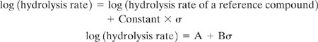
where σ is a structural parameter commonly used in linear free energy relationships, the Hammet constant. The Hammet constant characterizes the electron donating or electron withdrawing properties of a functional group. The details of estimating the Hammet constant and other parameters used in hydrolysis rate estimations are beyond the scope of this chapter, and it should be noted that empirical values for the constants A and B in Equation 5-22 must be determined for individual classes of reactants (e.g., the values for esters would be different than the values for epoxides). The parameter A is reaction and compound class specific because it depends on the reference reaction chosen. The parameter B is reaction and compound class specific because the dependence of rate on structural features depends on the type of reaction being considered.
Table 5.3-3 Group Contributions for Rate Constants for Hydroxyl Radical Additions to (C=C=C–) (Kwok and Atkinson, 1995).
An added complexity is that rates of reactions, such as hydrolysis, depend not just on the structure of the reactant, but also on the characteristics (e.g., pH) of the receiving waters. Thus, an estimate of hydrolysis rates requires both good rate estimation methods—which are scarce—and a detailed understanding of local environmental conditions.
5.3.3 Estimating Overall Biodegradability
In addition to all of the reactions that may occur with other chemicals in the atmosphere and in aqueous environments, we must also be concerned with the rate at which compounds are metabolized by living organisms. Developing an overall assessment of biodegradation will be difficult. Nevertheless, semi-quantitative assessments are possible. An ideal framework for estimating biodegradation would distinguish between the initial structural change of the compound (primary biodegradation) and the complete conversion to stable reaction products such as CO2 and H2O (ultimate biodegradation). It would also distinguish between aerobic (oxygen present) and anaerobic degradation.
Unfortunately, primary and ultimate, aerobic and anaerobic biodegradation rates are available for only a small number of compounds. Therefore, the approach described in previous sections—statistical regression of measured environmental data to yield group contribution parameters—will not work because there are not enough biodegradation data. Nevertheless, it is extremely important to have a qualitative sense of the persistence of compounds in the environment, and biodegradation is one of the most significant removal pathways for compounds in ambient environments. One pragmatic response to this problem has been to rely on estimations of biodegradation by expert panels. As described by Howard, et al. (1992) and Boethling, et al. (1994), expert panels can provide estimates of whether biodegradation occurs over hours, days, weeks, months or longer. These expert assessments can then be used as the basis for a group contribution method for biodegradation.
One such method (Boethling, et al., 1994) involves calculating an index that characterizes aerobic biodegradation rate in ambient environments.
![]()
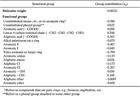
where I is an indicator of the aerobic biodegradation rate. A value of 5 indicates that the compound is expected to degrade over hours; a value of 4 corresponds to a lifetime of days; 3, 2 and 1 correspond to weeks, months, and longer, respectively. These values of I should not be viewed as an accurate quantitative predictor of biodegradation rate. Rather, they should be viewed as a relative ranking of the probability that a material will biodegrade. The parameter fn is the number of groups of type n in the molecule, and an is the contribution of group n to degradation rate. Group contribution parameters are listed in Table 5.3-4 and sample calculations are given in Example 5.3-4.
Estimate the biodegradation index for 1-propanol and diphenyl ether.
Solution: 1-propanol has a molecular weight of 60 and contains an aliphatic OH. Its biodegradation index is:
I = 3.199 + 0.160 – 0.00221(60) = 3.22
This implies a lifetime of weeks.
Diphenyl ether has a molecular weight of 170 and contains an aromatic ether and two mono-aromatic rings. Its biodegradation index is:
I = 3.199 + 2(0.022) – 0.058 – 0.00221(170) = 2.81
This implies a lifetime of weeks; literature data indicate a lifetime of months.
Table 5.3-4 Group Contributions to Ultimate Aerobic Biodegradation Index (Boethling, 1994).
Summary
This section has provided a limited introduction to methods for estimating environmental persistence. The methods are generally specific to a particular environmental medium (air, water, or sediment/soil) and to particular reaction pathways (e.g., reaction with hydroxyl radical in the atmosphere or hydrolysis in aqueous environments). Often the methods will depend on local characteristics, such as the acidity or alkalinity of a water body and the concentration of oxidizing species in the atmosphere. With all of these restrictions, the appropriate use of these methods in performing screening assessments is simply for relative rankings of environmental persistence.
Section 5.3 Questions For Discussion
1. When we examine atmospheric oxidation, we monitor only the disappearance of the chemical of interest. Should we be concerned about the reaction products that are formed?
2. The methodologies presented in this chapter represent only a small fraction of possible environmental degradation pathways. How would you use these limited data to perform an overall assessment of environmental persistence?
5.4 Estimating Ecosystem Risks
Structure activity relationships may also be used to assess ecosystem and human health impacts. The range and variety of such relationships are enormous. Therefore, this section will present only a few, simple relationships that are used to assess ecosystem risk. For a more comprehensive review, the interested reader is referred to extensive literature on structure activity relationships (e.g., Hansch, et al., 1995a,b), as well as extensive literature of experimental data (see, for example, online databases of the US EPA available at the EPA website: http://www.epa.gov, or the databases cited in Appendix F).
In assessing ecosystem hazard, the standard practice is to estimate toxicity for a variety of species. For example, mortality for daphnids, fish, and guppies are frequently used in assessing the ecosystem hazard of chemicals described in premanufacture notices submitted to the US EPA under the Toxic Substances Control Act. The mortality for guppies can be correlated with the octanol-water partition coefficient using Equation 5-24
![]()
where LC50 is the concentration that is lethal to 50% of the population over a 14-day exposure (expressed in mol/L). This equation was developed using data from a variety of different compounds, including chlorobenzenes, chlorotoluenes, chloroalkanes, diethyl ether, and acetone (Konemann, 1981). log 11>LC502 0.871 log Kow4.87
Other equations used to estimate ecosystem hazard are specific to certain compound classes. For example, toxicities for daphnids and fish can be estimated for more than 50 different compound classes. The correlations for acrylates are given below:
![]()
![]()
where LC50 is expressed in units of millimoles/L.
Example 5.4-1
Compare the fish, guppy and daphnid mortailities for an acrylate with log Kow=1.28 (e.g. methyl methacylate).
Solution: The concentrations yielding 50% mortality are:
Guppies (14 day): | 5690 μmol/L |
Daphnids (48 hour): | 0.226 millimoles/L = 226 μmol/L |
Fish (96 hour): | 0.020 millimoles/L = 20 μmol/L |
Section 5.4 Questions For Discussion
1. Why are ecotoxicities evaluated for immature amphibians and similar biota?
2. Why are the lethal concentrations negatively correlated with the octanol-water partition coefficient for these species?
5.5 Using Property Estimates to Estimate Environmental Fate and Exposure
The previous sections have described methods that can be used to estimate the properties that will govern a chemical’s environmental partitioning and fate. This section will illustrate, through a few simple examples, how those properties can be employed to estimate partitioning and fate. These properties will also be used in Chapter 6 to estimate exposures.
Consider, for example, the problem of estimating exposure to a chemical via inhalation. To calculate inhalation exposure, it is necessary to know atmospheric concentrations. Breathing rates are multiplied by atmospheric chemical concentrations to determine inhalation exposures. The atmospheric chemical concentration depends on emission rate, mixing rate, and atmospheric lifetime. A simple case study is given in Example 5.5-1.
Example 5.5-1
Propylene is emitted at a rate of 10 metric tons per year into an airshed that has a volume of 104 cubic kilometers. Assume that the airshed has a residence time of one day and is well mixed. Calculate the steady state concentration of propylene, accounting for chemical reaction. Calculate an inhalation exposure for an adult, assuming an inhalation rate of 20 l/min.
Solution: Perform a mass balance to calculate the steady state concentration of propylene:
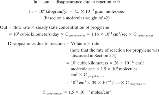
Assuming one mole of air occupies 22,400 cm3 at ambient conditions,
Cpropylene, ss = 3.3 × 10⁻¹³ moles propylene/mole air = 0.3 ppt
The exposure, assuming an inhalation rate of 20 L/min is:
20000 × 1.5 × 10-17 moles/cm3 = 30 × 10-14 moles/min = 6.6 × 10⁻⁶ g/yr
Far more sophisticated models than the well-mixed box model, used in Example 5.5-1, can be used to estimate atmospheric concentrations and inhalation rates. Many such models are available and calculating atmospheric concentrations, in order to estimate inhalation rates, is done relatively routinely. The problems associated with estimating environmental exposures via other routes become far more complex. Consider the relatively simple example of calculating exposure through drinking contaminated surface water. Assume that a chemical is released to a river upstream of the intake to a public drinking water treatment plant. To evaluate the exposure we would need to determine:
• What fraction of the chemical was adsorbed by river sediments?
• What fraction of the chemical was volatilized to the atmosphere?
• What fraction of the chemical was taken up by living organisms?
• What fraction of the chemical was biodegraded or was lost through other reactions?
• What fraction of the chemical was removed by the treatment processes in the public water system?
Thus, exposure estimates will require information on the soil sorption coefficient, vapor pressure, water solubility, bioconcentration factor, and biodegradability of the compound, as well as river flow rates, surface area, sediment concentration and other parameters. A simple, yet typical, set of calculations is shown in Examples 5.5-2 through 5.5-4.
Example 5.5-2
Assume that a chemical, with a molecular weight of 150, is released at a rate of 300 kg/day to a river, 100 km upstream of the intake to a public water system. Estimate the initial partitioning of the chemical in the water, sediment, and biota.
Data
Water solubility: 100 ppm
Soil sorption coefficient: 10,000
Organic solids concentration in suspended solids: 15 ppm
River flow rate: 500 million liters per day
Bioconcentration factor: 100,000
Biota loading: 100 g per 1000 cubic meter
Solution: The ratio of concentrations in water, sediment and biota will be approximately:
1:10,000:100,000
Based on the river flow rate, the total flow rates of water, sediment, and biota are:
Water: (500 million liter/day × 1 kg/liter)=500 million kg/day
Sediment: 500 million kg/day × 15 kg sediment/million kg water= 7500 kg sediment/day
Biota: 500 million kg/day × 0.1 kg biota/million kg water 50 kg biota/day
Performing a mass balance:

where (Cwater) is the chemical concentration in the water phase:
(Cwater=0.5 ×10⁻⁶kg chemical/kg water= 0.5 ppm
This is well below the solubility of 100 ppm. The ratio of the mass in water, sediment, and biota is:
500,000,000:75,000,000:5,000,000
86:13:1
Thus, although the concentrations are much higher in the biota and the sediment, more than 80% of the mass remains in the water phase.
Example 5.5-3
For the discharge described in Example 5.5-2, calculate the equilibrium partial pressure of the chemical above the river at the discharge point. Is volatilization from the river likely to be significant?
Data
Vapor pressure: 10-1 mm Hg
River flow rate: 500 million liters per day
River velocity: 0.5 m/sec
River width: 30 m
Solution: Assuming ideal behavior and the concentration determined in Example 5.5-2, the equilibrium vapor pressure should be:
0.5 × 10⁻⁶ g chemical/g water × 1 mole chemical/150 g ×
18g/mole water × 10-1 mm Hg = 0.6 × 10⁻⁹ mmHg = 8.0 × 10⁻¹² atm
To determine if the loss rate is significant, assume that a volume 10 m above the river reached this concentration for the length of the river to the public water system inlet (a total volume of 100,000 10 30 m3). Noting that 1 gram-mole of air at standard conditions occupies 22.4 liters:
30 × 106 × m3 (1 mole air/0.0224 m3)× 8.0 × 10-12 moles chemical/mole air ×
150 g/mole = 1.6 g
This is the mass required to saturate the atmosphere to a height of 10 m above the river for the 100 km length of the river. Compare this to the total discharge rate of 300 kg/day, and it is clear that volatilization will be negligible.
Example 5.5-4
For the discharge described in Examples 5.5-2 and 5.5-3, estimate what fraction of the initial discharge might still be in the water at the public water intake. If the treatment efficiency of this chemical in the water treatment plant is 95%, what would be the concentration in drinking water?
Data
Biodegradation half life: 300 hours
Solution: Based on a river velocity of 0.5 m/sec and a travel distance of 100 km, the transit time is 2.3 days. If the half life is 300 hours, the disappearance rate constant is (see Example 5.3-1):
This can be used to calculate the ratio of final to initial concentration:
![]()
The concentration entering the treatment plant is 0.88 × 0.5 ppm.
The concentration in the drinking water is 0.05 × 0.88 × 0.5 ppm = 20 ppb.
Summary
The purpose of this section has been to illustrate how the properties evaluated in Sections 5.2 and 5.3 can be used to estimate environmental partitioning. Again, the models presented have been simple, demonstrating basic concepts of environmental partitioning, fate, and exposure. More complex and accurate models are available, but are beyond the scope of these simple screening methods.
Section 5.5 Questions For Discussion
1. Why is most of the mass of the chemical considered in Example 5.5-2 in the water phase, while the concentrations in the sediment and biota phases are so high?
2. For Example 5.5-3, what vapor pressure would result in significant volatilization rates?
3. How would you develop an accurate estimate for volatilization rate in Example 5.5-3 if the losses were significant?
5.6 Classifying Environmental Risks Based On Chemical Structure
The previous sections have described procedures for estimating the chemical and physical properties that are needed to assess potential environmental risks for chemicals. Our goals in this section are to put these property values in perspective and to introduce the tools that will be needed to perform an overall assessment of environmental hazards.
Three types of criteria are typically considered in risk-based evaluations— persistence, bioaccumulation and toxicity. For any one of these criteria, it may be necessary to consider a number of properties in performing an evaluation. For example, in evaluating persistence, it may be necessary to consider atmospheric halflives and biodegradation half-lives. In evaluating toxicity, it may be necessary to consider a variety of eco-toxicity measures and human toxicity measures. Because there is such a wide variety of criteria that can be used in evaluating environmental risks—ranging from human carcinogenicity to biodiversity—and because opinions vary widely on the relative importance of the evaluation criteria, there is no single evaluation methodology that is universally accepted for evaluating the environmental hazards of chemicals.
Therefore, our approach in this text will be to present approximate classifications that can be used to categorize chemicals according to their persistence, bioaccumulation potential, and toxicity. The classifications will group chemicals into categories of high, moderate, and low concern, using values established by the US EPA in evaluating chemicals under the Toxic Substances Control Act. For example, Table 5.6-1 is a summary of the categories used to classify the persistence and bioaccumulation of chemicals and Figure 5.6-1 shows distributions of one measure of ecotoxicity.
These qualitative screenings can be useful in assigning areas of concern. Ranking risks, however, is more problematic, and approximate methods for ranking chemical risks will be described in Chapter 8. For now, Table 5.6-1 and Figure 5.6-1 can be used to provide perspective on the values for properties generated using the methods of Sections 5-2 and 5-3.
Table 5.6-1 Classification Criteria for Persistence and Bioaccumulation.
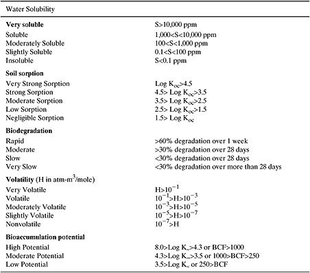
Figure 5.6-1 Distributions of measures of eco-toxicity for several thousand compounds. These distributions can be used to classify compounds into categories of concern. (Note that a high effect concentration implies that a large amount of the material can be released before an effect is observed.) (Zeeman, et al., 1993)

References
Atkinson, R. and Carter, W.P.L. 1984, “Kinetics and mechanisms of the gas-phase reactions of ozone with organic compounds under atmospheric conditions,” Chem. Rev. 84: 437–470.
Atkinson, R. 1985, “Kinetics and mechanisms of the gas-phase reactions of the hydroxyl radical with organic compounds under atmospheric conditions,” Chem. Rev. 85: 69–201.
Atkinson, R. 1986, “Estimations of OH radical rate constants from H-atom abstraction from C-H and O-H bonds over the temperature range 250-1000 K,” Intern. J. Chem. Kinet. 18: 555–568.
Atkinson, R. 1988, “Estimation of gas-phase hydroxyl radical rate constants for organic chemicals,” Environ. Toxicol. Chem. 7: 435–442.
Atkinson, R. 1987, “A structure-activity relationship for the estimation of rate constants for the gas-phase reactions of OH radicals with organic compounds,”Intern. J. Chem. Kinet. 19: 799–828.
Atkinson, R. 1989. “Kinetics and mechanisms of the gas-phase reactions of the hydroxyl radical with organic compounds,”J. Phys. Chem. Ref. Data Monograph No. 1, NY: Amer. Inst. Physics & Amer. Chem Soc.
Hansch, C., Leo, A. and Hoekman, eds., “Exploring QSAR: Volume 1, Fundamentals and Applications in Chemistry and Biology,” American Chemical Society, Washington, D.C., 1995a.
Hansch, C., Leo, A. and Hoekman, eds., “Exploring QSAR: Volume 2, Hydrophobic, Electronic and Steric Constants,” American Chemical Society, Washington, D.C., 1995b.
Howard, P.H., Handbook of Environmental Fate and Exposure Data for Organic Chemicals, Lewis Publishers, Chelsea, Mich., 1997.
Howard, P.H., Boethling, R.S., Stiteler, W.M., Meylan, W.M., Hueber, A.E., Beauman, J.A., and Larosche, M.E., “Predictive model for aerobic biodegradability developed from a file of evaluated biodegradation data,” Environmental Toxicology and Chemistry, 11, 593–603 (1992).
Joback, K.G. and Reid, R.C., “Estimation of Pure-Component Properties from Group Contributions,” Chemical Engineering Communications, 57, 233–243 (1987).
Koneman, H. 1981, “Fish toxicity tests with mixtures of more than two chemicals: a proposal for a quantitative approach and experimental results,” Toxicology 19: 229–238.
Kwok, E.S.C. and Atkinson, R. 1995, “Estimation of Hydroxyl Radical Reaction Rate Constants for Gas-Phase Organic Compounds Using a Structure-Reactivity Relationship: An Update,” Atmospheric Environment (29: 1685-95). [from Final Report to CMA Contract No. ARC-8.0-OR, Statewide Air Pollution Research Center, Univ. of CA, Riverside, CA 92521].
Lyman, W.J., “Estimation of Physical Properties,”Environmental Exposure from Chemicals Volume 1, Neely, W.B. and Blau, G.E., eds., CRC Press, Boca Raton, FL 38-44 (1985).
Lyman, W.J., Reehl, W.F. and Rosenblatt, D.H., eds, Handbook of Chemical and Physical Property Estimation Methods: Environmental Behavior of Organic Compounds, American Chemical Society, Washington, D.C., 1990.
Mackay, D., Shiu, W.Y., and Ma, K.C., Illustrated Handbook of physical-chemical properties and environmental fate for organic chemicals, Lewis Publishers, Boca Raton, 1992.
Meylan, W.M. and Howard, P.H., “Bond Contribution Method for Estimating Henry’s Law Constants,” Environmental Toxicology and Chemistry, 10, 1283–1293 (1991).
Meylan, W.M., Howard, P.H., and Boethling, R.S., “Molecular Topology/Fragment Contribution Method for Predicting Soil Sorption Coefficients,”Environ. Sci. Technol., 26, 1560–1567 (1992).
Meylan, W.M. and Howard, P.H., “Atom/Fragment Contribution Method for Estimating Octanol-Water Partition Coefficients,” Journal of Pharmaceutical Sciences, 84, 83–92 (1995).
Meylan, W.M., Howard, P.H., and Boethling, R.S., “Improved Method for Estimating Water Solubility from Octanol/Water Partition Coefficient,” Environmental Toxicology and Chemistry, 15, 100–106 (1996).
Mill, T., Haag, W., Penwell, P., Pettit, T., and Johnson, H. “Environmental Fate and Exposure Studies Development of a PC-SAR for Hydrolysis: Esters, Alkyl Halides and Epoxides,” EPA Contract 68-02-4254. Menlo Park, Ca.: SRI International (1987).
Reid, R.C., Prausnitz, J.M., and Sherwood, T.K., The Properties of Gases and Liquids, 4th ed., McGraw Hill, 1987.
Reinhard, M. and Drefahl, A., Handbook for Estimating Physicochemical Properties of Organic Compounds, Wiley, New York, 1999.
Seinfeld, J.H. and Pandis, S. N., Atmospheric Chemistry and Physics, Wiley Interscience, New York, 1998.
Stein, S.E. and Brown, R.L., “Estimation of Normal Boiling Points from Group Contributions,” J. Chem. Inf. Comput. Sci., 34, 581–587 (1994).
Zeeman, M., Clements, R.G., Nabholz, J.V., Johnson, D. and Kim, A., “SAR/QSAR Ecological Assessment at EPA/OPPT: Ecotoxicity Screening of the TSCA Inventory,” Society of Environmental Toxicology and Chemistry Annual Meeting, Houston, November, 1993.
Problems
Use the methods described in the chapter. In addition, available software to estimate these properties may be used. (http://www.epa.gov/oppt/exposure/docs/episuite.htm)
1. Estimate the properties listed in the table given below.

2. Estimate the properties listed in the table given below. If group contributions are not available for the necessary groups, use reasonable judgment in estimating parameters.
3. Estimate the properties listed in the table given below.


For each of the properties, comment on whether molecular weight or the presence of a hydrogen bonding group has a more pronounced effect on chemical properties.
4. Benzene in the wastewaters from a manufacturing facility is sent, at a rate of 2000 kg/day, to a publicly owned wastewater treatment works (POTW). The POTW treats the benzene in the wastewater and removes 85% of the organic before discharging to a local river. One hundred kilometers downriver of the discharge point is the intake to a public water system.
Data
River flow rate: 1250 million liter per day
River velocity: 0.5 m/sec
River width: 50 m
Organic solids concentration in suspended sediment: 15 ppm
Biota concentration: 100 g per 100 cubic meter
(a) Estimate the fraction of benzene in water, sediment, and biotic phases at the dis-charge point.
(b) Determine whether volatilization of benzene from the river is likely to be signifi-cant.
(c) Estimate the fraction of the benzene that biodegrades before the effluent reaches the water intake.
(d) Estimate the potential toxicity of the releases to aquatic life.
5. During pesticide application, 1 kg of hexachlorobenzene is accidentally applied to a 108 liter pond. Estimate the amount of hexachlorobenzene that would be ingested if a person were to eat a 0.5 kg fish from the pond. Assume that the pond is well mixed and that the organic sediment content is 10 ppm and the total fish loading is 100 g per 100 cubic meter.
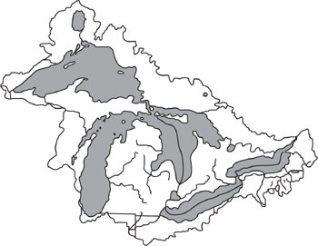
6. The Great Lakes Basin is one of the largest freshwater ecosystems in the world. Recently there has been some concern that persistent, bioaccumulative and toxic compounds have been accumulating in the basin, possibly compromising this valuable natural resource. Of particular concern are the chlorinated organics. In 1993 (the most recent year for which data are available) the chlorinated organic released in greatest quantity in the Great Lakes Basin was tetrachloroethylene. The emission rates to air, land and water for the basin were 1.8 × 10⁷ pounds per year, 2.6 × 10⁶ pounds per year and 8.4 × 10² pounds per year, respectively.
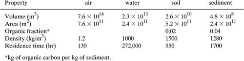
(a) Calculate the equilibrium partitioning of tetrachloroethylene in the air, water, soil and sediment of the Great Lakes Basin. Use one year of emissions as your basis. Assume no degradation, initial concentrations are zero, and that the Great Lakes Basin has the properties listed below.
(b) Will the system that you modeled in part (a) ever reach a steady state? Explain your reasoning.
(c) Estimate the atmospheric half-life and the biodegradability of tetrachloroethylene. Based on these values, estimate the steady state concentration of tetrachloroethylene in each environmental compartment.
Hint: for steady state to be reached, the total mass input to the systems must equal the total mass lost due to reaction. Assume that biodegradation occurs in water, sediment and soils and that degradation occurs in the atmosphere. Set up a mass balance where you have only one concentration as an independent variable and solve for that concentration.)
(d) In parts a–c you assumed that the environmental compartments were closed (e.g., you effectively assumed that the atmosphere was not ventilated by winds from other regions). Now assume that you want to account for advection in your calculation of steady state concentrations. Describe qualitatively how you would include the atmospheric, water, soil and sediment residence time information provided in the Table for Part (a) into your analysis. Use equations in your explanation if you wish, but do not attempt a quantitative analysis.
7. Design a solvent molecule that has a vapor pressure greater than 1 mm Hg, a molecular weight between 75 and 150, and will biodegrade in less than one month.
8. Design a solvent molecule that has a vapor pressure less than 1 mm Hg (at 300 K), a molecular weight between 75 and 150, and will biodegrade in less than one month.
9. The group contribution equation for estimating boiling point is:
Tb = 198.2 + ∑ni gi
Without consulting the tables in Chapter 5, estimate the relative magnitude of the group contributions for the following three functional groups: –OH, –CH3, –Cl(aliphatic). Report your answer as x<y<z, where x, y, and z are the three functional groups. For example if you believed that the values of the three group contributions for –OH, –CH3, –Cl were 1, 0 and 1, respectively, your answer would be OH< CH3< Cl.Explain your reasoning.
10. Without consulting the tables in Chapter 5, estimate the relative magnitude of the group contributions for octanol-water partition coefficient for the following three functional groups: –OH, –CH3, –Cl (aliphatic). Report your answer as x<y<z, where x, y, and z are the three functional groups. For example if you believed that the values of the three group contributions for –OH, –CH3, –Cl were –1, 0 and 1, respectively, your answer would be –OH< –CH3< –Cl.Explain your reasoning.