Chapter 11
Evaluating the Environmental Performance of a Flowsheet

by
David R. Shonnard

11.1 Introduction

After the process flowsheet has been established and energy and mass efficiency measures have been applied (Chapter 10), it is appropriate for a detailed environmental impact evaluation to be performed. The end result of the impact evaluation will be a set of environmental metrics (indexes) which represent the major environmental impacts or risks of the entire process. A number of indexes are needed to account for potential damage to human health and to several important environmental media. The indexes can be used in several important engineering applications during process design, including the ranking of technologies, the optimizing of in-process waste recycle/recovery processes, and the evaluation of the modes of reactor operation.

In quantitative risk assessment, it is shown that impacts are a function of dose, that dose is a function of concentration, and that concentration is a function of emission rate. Therefore, emissions from a process design flowsheet are the primary piece of information required for impact assessment. The concentrations in the relevant compartments of the environment (air, water, soil) are dependent upon the emissions and the location and chemical and physical properties of the pollutants. A suitable fate and transport model can transform the emissions into environmental concentrations. Finally, information regarding toxicity or inherent impact is required to convert the concentration-dependent doses into probabilities of harm (risk). Based on this understanding of risk assessment, the steps for environmental impact assessment are grouped into three categories, a) estimates of the rates of release for all chemicals in the process, b) calculation of environmental fate and transport and environmental concentrations, and c) the accounting for multiple measures of risk using toxicology and inherent environmental impact information.

Ideally, one would prefer to conduct a quantitative risk assessment when comparing the environmental performance of chemical process designs. Although this approach is preferred when the source and receptor are well defined and localized, it is not well suited for industrial releases that often affect not only local, but also regional and global environments. Also, the computing resources needed to perform a quantitative risk assessment for all release sources and receptors would tax the abilities of even the largest chemical manufacturer. A more achievable approach is to abandon quantitative risk assessment in preference to the assessment of potential environmental and health risks. The establishment of the potential impacts of chemical releases is sufficient for comparing the environmental risks of chemical process designs. In this chapter, material is presented which establishes methodologies for assessing the potential for environmental impacts of chemical processes and their designs.

In this development, we will utilize the concept of impact benchmarking. First introduced for the assessment of global warming and ozone-depletion potentials of refrigerants in the early 1990s, benchmarking takes the ratio of the environmental impact of a chemical’s release to the impact of the identical release of a wellstudied compound. A value greater than 1 for this dimensionless quantity indicates that the chemical has a greater potential for environmental impact than the benchmark compound. The product of the benchmarked environmental impact potential with the process emission rate results in the equivalent emission of the benchmark compound in terms of environmental impact. In this text, we adopt the benchmarking concept when assessing the environmental and toxicological impact potentials of releases from chemical processes. (Heijungs et. al. 1992)

Section 11.2 is a description of a multimedia compartment model approach for determining fate and transport of chemical releases into the environment. This model predicts the long-time and large-spatial scale distribution of chemicals using multiple compartments as the physical structure for the environment. Section 11.3 is a presentation of a Tier 3 environmental assessment (Tier 1 and Tier 2 assessments are discussed in Chapter 8) consistent with the goal of efficiently comparing chemical process designs.

11.2 Estimation of Environmental Fates of Emissions and Wastes

After a chemical is released into a compartment of the environment, either to the air, the surface water, or the soil, there are several transport and reaction processes that affect the ultimate concentrations in each of these compartments. There is also more than one modeling approach for calculating these concentrations.

Two important issues arise when choosing the type of environmental fate and transport model—accuracy and ease of use. Accuracy depends on how rigorously the model incorporates environmental processes into its description of mass transport and reaction. Ease of use relates to the data requirements and computational demands which the model places on the environmental assessment. One very common modeling approach used in environmental applications focuses on transport and fate processes occurring on only one compartment. The familiar atmospheric dispersion models for predicting air concentrations downwind from stationary sources (stacks) are examples of these single compartment models (Seinfeld and Pandis, 1997; Thibodeaux, 1996). Other very important examples are groundwater dispersion models that are used to predict concentration profiles in contaminated plumes downgrading from subsurface pollution sources (Fetter, 1993). The advantages of these models are that they require little chemical and environmentalspecific data and provide relatively accurate results using modest computer resources. The disadvantage is that they provide concentration information in only one compartment, a severe limitation when multiple environmental impacts are under consideration. Several single compartment models can be linked together, thus providing multi-compartmental (multimedia) insights into environmental fate and transport. Unfortunately, the computational requirements are very large, making practical implementation difficult for routine chemical process evaluation.

The second major modeling approach is to use multimedia compartment models (MCMs), which predict chemical concentrations in several environmental compartments simultaneously (Mackay, 2001; McKone, 1994; Cohen et al., 1990). The advantages of MCMs are that they require modest data input, they are relatively simple and computationally efficient, and they account for several intermediate transport mechanisms and degradation. Limitations include a general lack of experimental data that can be used to verify their accuracy, and the general belief that they can provide only order-of-magnitude estimates of environmental concentrations (Mackay and Paterson, 1991). Keeping these limitations in mind, we present and demonstrate with example problems the Level III multimedia fugacity model of Mackay (2001). This model predicts the steady-state concentrations of a chemical in four environmental compartments (air (1), surface water (2), soil (3), and sediment (4)) in response to a constant emission into an environmental region of defined volume. The numbering convention used above for the compartments will be followed in the remainder of the text.

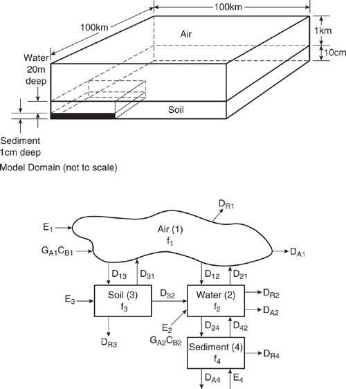
The surface area selected for the model is 10⁵ km², about the area of Ohio, Greece, or England. The fraction of the area covered by water and by soil is a region-specific value, but typical values of 10% water and 90% land are often used (Mackay, 2001). The surface area of sediment is the same as the water compartment surface area. The atmosphere height is set at 1000 m, which is the typical height affected by pollutants emitted at the earth’s surface. The depth of the water compartment is 20 m and those of the soil and sediment layers are assumed to be 10 cm and 1 cm, respectively. The atmosphere compartment contains a condensed (aerosol) phase having a volume fraction in air of 2×10^-11 or about 30 µg/m³. Though the aerosol phase is present in only a small amount, a large fraction of a chemical in the air may be associated with aerosols. The water compartment contains suspended sediments of volume fraction 5×10^-6 (5 mg/L) and organic carbon content of 20%. Fish are included at a volume fraction of 10^-6 and are assumed to contain 5% lipid into which hydrophobic chemical can partition. The soil compartment is assumed to contain 20% by volume of air, 30% water, and the remainder solids. The organic carbon content of soils is 2%. All of these parameters could be modified, if appropriate, but these values are reasonable and will be used in the examples presented in this chapter.

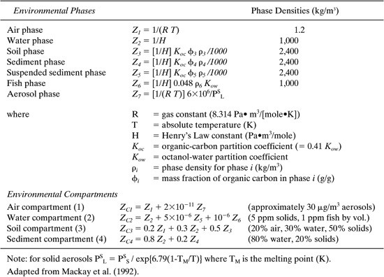
Figure 11.2-1 is a schematic diagram of the chemical processes occurring in the model domain which can affect the concentrations in each of the four compartments. Chemical may directly enter compartments by emissions (E_i) (moles/hr) and advective inputs (G_AiC_Bi) (moles/hr). There is transfer of chemical between compartments by diffusive and non-diffusive processes characterized by intermediate transfer values (D_ij) (moles/(Pa•hr)). Chemical may enter or exit compartments by advective (bulk flow) mechanisms having a transfer value D_Ai, and chemical may disappear by reaction within each compartment having a loss value of D_Ri.

MCMs use the concept of fugacity in describing mass transfer and reaction processes. Fugacity is a thermodynamic property of a chemical and is defined as the “escaping tendency” of the chemical from a given environmental phase (air, water, soil organic matter, etc.). Thus for example, a volatile organic compound having a low water solubility will exhibit a large escaping tendency from the water phase (large water fugacity). Partitioning of a chemical between environmental phases can be described by the equilibrium criterion of equal fugacity f (Pa) in all phases. The fugacity is equal to partial pressure in the dilute limit typical of most environmental concentrations. Another feature of fugacity is that it is generally proportional to concentration, C = fZ, where Z is termed the fugacity capacity (Pa•m³/mole) and C is the concentration (mole/m³).

It is illustrative to develop expressions for relating fugacity to concentration in different environmental phases. We analyze seven phases: air, water, solids (soil, sediment, and suspended sediment), fish, and aerosol. Following that, we present several prominent intermediate transport mechanisms and reaction expressions for inclusion in the model. Finally, the model equations are presented and solved for the fugacity and ultimately the molar concentrations in each compartment.

11.2.1 Fugacity and Fugacity Capacity

Air Phase (1). The fugacity in the air phase is rigorously defined as

f = y φ P_T ≈ P

where y is the mole fraction of the chemical in the air phase, φ is the fugacity coefficient (dimensionless) which accounts for non-ideal behavior, and P_T is the total pressure (Pa). At the relatively low pressures (1 atm) encountered in the environment, φ = 1, making the fugacity equal to the partial pressure (P) of the chemical in air. The concentration is related to partial pressure (and fugacity) by the ideal gas law, where n is moles of the chemical ina volume V (m³), R is the gas constant (8.31 Pa•m³/[mole•K]), and T is the absolute temperature (K). The air phase fugacity capacity Z₁ is 1/RT and has value of 4.04×10^-4 moles/(m³•Pa) at 25°C. The fugacity capacity is shown to be independent of chemical, being a constant value at a constant system temperature.

C₁ = n/V = P/(RT)= f/(RT) = fZ₁

Figure 11.2-1 Schematic diagram of fugacity level III model domain and the intermedia transport mechanisms.

Water Phase (2). In aqueous solution, the fugacity of a chemical is

f = xγ P^s

where x is the mole fraction, γ is the activity coefficient in the Raoult’s Law convention, and P^s is the saturation vapor pressure of pure liquid chemical at the system temperature (Pa). It can be shown that in most situations involving dilute concentrations typical of environmental problems, the activity coefficient is a constant (not varying with concentration (x)). Thus, there is a linear relationship between f and concentration in aqueous solution, C₂ (moles/m³). Rearranging the equation above results in the desired relationship,

C₂ = x/v_w = f/(v_wγP^s = f/H = fZ₂

where ν_w is the molar volume of solution (water, 1.8×10^-5 m³/mole), H is the Henry’s Law constant for the chemical (Pa• m³/mole), and Z₂ is the water fugacity capacity for each chemical, which is the inverse of the chemical’s Henry’s Law constant.

Soil Phase (3). Chemicals associated with the soil or sediment phases are almost always sorbed into the natural organic matter in the soil and are in equilibrium with the water phase concentration. A linear relationship has been observed between the sorbed concentration (C_s, moles/kg soil or sediment) and the aqueous concentration (C₂, moles/L solution).

C_s = K_dC₂

where K_d is the equilibrium distribution coefficient (L solution /kg solids) and the slope of the linear sorption isotherm. Because natural organic matter is composed mainly of carbon, the distribution coefficient is related to the fraction of organic carbon in the soil or sediment by

K_oc = K_d/φ₃

where K_oc is the organic carbon-based distribution coefficient (L/kg) and φ₃ is the mass fraction of organic carbon in the soil phase (g organic carbon/g soil solids). The octanol-water partition coefficient has been shown to correlate very well with K_oc with the equality K_oc = 0.41 K_ow being a good approximation for most chemicals (for other estimation methods, see Chapter 5). We find it convenient to relate the concentration per volume of the sorbed phase (C₃ for soil solids) to the fugacity by multiplying C_s by the phase density (_ρ3, kg solid/m³ solid) and by relating C₂ to partial pressure (fugacity) through the Henry’s Law constant.

Thus:

_ρ3 C₃ = [1/H] K_oc φ_{3 ρ3} f/1000 = Z₃f

where the factor of 1000 is used to convert L to m³.

Similar expressions for fugacity capacities (Z) are obtained for the other environmental phases which make up the four environmental compartments. A sum-mary of these equations is given in Table 11.2-1. Included in Table 11.2-1 are the fugacity capacities for each of the environmental compartments—the air, surface water, soils, and sediments—which are summations of individual phase Z values weighted by their respective volume fractions in the compartment.

Table 11.2-1 Fugacity Capacity (Z) Values for the Various Phases and Compartments in the Environment.

11.2.2 Intermedia Transport

Chemicals move between environmental compartments by diffusive and nondiffusive processes. Diffusive processes, such as volatilization from water to air or soil to air, can proceed in more than one direction, depending on the sign of the fugacity difference between compartments. The diffusive rate of transfer N_ij (moles/h) from a compartment i to compartment j is defined by;

N_ij = D_ij(f_i) (moles/h)

where D_ij (mole/(Pa•hr)) is an intermedia transport parameter for diffusion from compartment i to j and f_i is the fugacity in compartment i, serving to drive the chemical into adjoining compartments. A comparable expression exists for the molar rate of transfer from compartment j to i. The difference in these molar rates is the net rate of transfer between these compartments due to a disequilibrium in the compartmental fugacities. In parallel to diffusive transport is non-diffusive (one-way) transport between compartments, such as rain washout and wet/dry deposition of atmospheric particles to soil and water, and sediment deposition and resuspension. This transport can be described by

N = GC = GZf = Df (moles/h)

where G (m³/h) is a volumetric flow rate of the transported material (rainwater, suspended sediment, etc.) and C (moles/m³) is its phase concentration. Figure 11.2-1 illustrates all of the intermediate diffusive and non-diffusive transport mechanisms within the model domain. In the following discussion, each intermediate transport parameter will be derived.

Air/Water Transport (D₁₂ and D₂₁)

Three processes are included in air-to-water transport: diffusion (absorption), washout by rain, and wet/dry deposition of aerosols. The conventional two-film approach is taken for absorption from air to water compartments through the atmosphere/water interface using air-side (k_A = 5 m/h) and water-side (k_W = 0.05 m/h) mass transfer coefficients. For the sake of organization, we rename the mass transfer coefficients as k_A = u₁ and k_W = u₂ and follow this convention for the remaining derivations. The intermediate transport parameter for absorption is

D_vw = 1/(1/(u₁A_wZ₁) + 1/(u₂A_wZ₂))

where A_w is the interfacial area between the atmosphere and the surface water. For rain washout, a rainfall rate u₃ of 0.876 m/yr (10^-4 m/h) is assumed. The value for rain washout is

D_RW = u₃A_wZ₂

For wet and dry deposition of aerosols, the deposition velocity u₄ is taken to be the sum of these parallel transport mechanisms (6×10^-10 m/h) and therefore the D value becomes.

D_QW = u₄A_wZ₇

Since these mechanisms operate in parallel, we can define a cumulative D value for the air-to-water transfer (D₁₂)as

D₁₂ = D_vw + D_RW + D_QW

The water-to-air transport is just the reverse of the absorption mechanism described above and therefore, the D value for water-to-air transport (D₂₁) is

D₁₂ = D_vw

Air-Soil Transport (D₁₃ and D₃₁)

For air-to-soil transport, identical treatments of rain washout (D_RS) and wet/dry deposition (D_QS) are taken as in the air-to-water transport case. The only difference is that the correct area term is the air/soil interface area, A_S. For diffusion from air to soil, the chemical must traverse a thin mass-transfer resistance film at the atmosphere/soil interface before diffusing through the soil air phase or the soil water phase, both of which have resistances of their own. The value of this mass transfer coefficient at the soil surface u₅ is the same as the air-side mass transfer coefficient for the atmosphere-water interface u₁ (5 m/h). Diffusion through the soil air or water phases is hampered by the presence of the soil solids, and as a result, the molecular diffusion coefficients of the chemical in either air or water decreases substantially. The Millington-Quirk relationship is employed as outlined in the work by Jury et al. (1983, 1984) to decrease the diffusion coefficients by a factor of about 20. Thus, the effective air diffusion coefficient becomes 0.05 * 0.02 m²/h = 10^-3 m²/h and the effective water diffusion coefficient becomes 0.05 * 2×10^-6 m²/h = 10^-7 m²/h. The effective diffusion coefficients divided by the path length for diffusion in soil (half the soil depth, 0.05 m) yields the mass-transfer coefficients for diffusion in the soil water u6 = 2×10^-6 m/h and soil air u₇ = 0.02 m/h. Downward flow of water in the soil pores is likely to result in a water transport velocity of about 10^-5 m/h. Thus, u₆ is taken to be a larger value in order to account for this, 10^-5 m/h. The soil diffusion processes in the air and water occur in parallel but are in series with the air film at the soil surface. The final equation for air-to-soil diffusion D value is

D_vs = 1/(1/D_s + 1/(D_sw + D_SA))

where

D_s = u₅A_sZ₁

D_sw = u₆A_sZ₂

D_SA = u₇A_sZ₁

The total D value for all air-to-soil processes is given by

D₁₃ = D_vs + D_QS + D_RS

For soil-to-air diffusion transport, the D₃₁ value is equal to D_VS.

Water-Sediment Transport (D₂₄ and D ₄₂)

Diffusion from the water column to the sediment is characterized by a masstransfer coefficient u₈ or 10^-4 m/h, which is the molecular diffusivity in water (2×10^-6 m²/h) divided by the path length (0.02 m). Ignored are the processes of bioturbation and shallow water current-induced turbulence which would increase u₈. The D value is u₈A_WZ₂. Deposition of suspended sediment is assumed to occur at a rate of 5000 m³/h over an area A_W = 10¹⁰ m². Thus the suspended sediment deposition velocity u₉ is 5000 m³/h/A_W = 5×10^-7 m/h. The water to sediment D value is thus

D₂₄ = u₈A_wZ₂ + u₉A_wZ₅

where Z₅ is the Z value for the suspended sediment.

Sediment to water is treated similarly to D₂₄. Resuspension is assumed to occur at a rate which is 40% that of deposition. Therefore, the resuspension velocity u₁₀ is 2×10^-7 m/h and the D value for sediment to water transfer is

D = u₈A_wZ₂ = u₁₀A_wZ₄

Soil to water (D₃₂)

Soil-to-water transfer occurs by surface run-off. The rate of water run-off is assumed to occur at 50% the rate of rainfall. The run-off water velocity u₁₁ is then 0.5 u₃ = 5×10^-5 m/h. The solids contained in the run-off water are assumed to be at a volumetric concentration of 200 ppm in the water. The run-off solids velocity u₁₂ is 200×10^-6u₁₁. The D value is

D₃₂ = u₁₁A_sZ₂ + u₁₂A_sZ₃

where A_S is the soil surface area and Z₂ is the Z value for the water and Z₃1 is the Z value for the soil solids. A summary of the intermediate transport parameters is shown in Table 11.2-2.

An additional non-diffusive transport mechanism which removes chemical from the sediment is burial. The D value (D_A4)is equal to

D_A4 = u_BA_WZ₄,

Where u_B is the sediment burial rate (2×10^-7 m/h).

Advective Transport

Chemical may directly enter into compartments by emissions and advective inputs from outside the model region. The total rate of inputs for each compartment i is

I_i = E_i + G_AiC_Bi

where E_i (moles/h) is the emission rate, G_Ai (m³/h) is the advective flow rate, and C_Bi (moles/m³) is the background concentration external to compartment i. Chemicals may also exit the model domain from compartments by advective (bulk flow) processes having transfer values (D_Ai)

Table 11.2-2 Intermedia Diffusive and Non-Diffusive Mass Transfer Coefficients (meters/hr).

D_Ai = G_AiZ_Ci

where Z_Ci is the compartment i fugacity capacity (Table 11.2-1).

11.2.3 Reaction Loss Processes

Reaction processes occurring in the environment include biodegradation, photolysis, hydrolysis, and oxidation. A good approximation for reaction processes in the dilute limit commonly found in the environment is to express them as first order with rate constant k_R (hr^-1). The rate of reaction loss for a chemical in a compartment N_Ri (moles/hr) is

N_Ri = k_RiV_iC_i = k_RiV_iZ_Cif = D_Rif

V_i is the compartment volume, C_i is the molar concentration of the chemical, and i refers to a specific compartment. Rate constants are compound-specific and have been tabulated for several compounds in the form of a reaction half-life t_1/2, defined as the time required for the concentration to be reduced by one half of the initial by reaction (Mackay et al., 1992; also see Chapter 5). Tabulated half lives for compounds might represent the combined reaction mechanisms listed above, which can occur simultaneously in a given compartment. The relationship between t_1/2 and k_R for a first order reaction is

k_R = – ln(0.5)/t_1/2

A summary of the D values for intermedia transport, advection, and reaction is shown in Table 11.2-3.

Table 11.2-3 D Values in the Mackay Level III Model (Adapted from Mackay and Paterson, 1991).

Table 11.2-4 Mole Balance Equations for the Mackay Level III Fugacity Model.

11.2.4 Balance Equations

As indicated in Figure 11.2-1, there must be a balance between the rates of input from all emissions/bulk flow and intermedia transport and the rates of output from intermedia transport, advection, and reaction loss processes within each compartment at steady-state. We write mole balance equations for each compartment as summarized in Table 11.2-4.

The fugacity calculations outlined in the previous pages are obviously very complex. Routine hand calculations of environmental fugacities using this model are prohibitively time consuming. Fortunately, spreadsheet programs are available for carrying out these calculations (Mackay et al., 1992, Volume 4). Using these programs and equipped with a relatively small number of chemical-specific input partitioning and reaction parameters, environmental fate calculations can be quickly performed as shown in the following example problem.

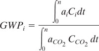
Example 11.2-1 Multimedia Concentrations of Benzene, Ethanol, and Pentachlorophenol.

Benzene, ethanol, and pentachlorophenol (PCP) are examples of organic pollutants with very different environmental properties, as shown in Table 11.2-5. Benzene and ethanol are volatile (high vapor pressures) and have comparatively short reaction half-lives. Pentachlorophenol has a long reaction half live, low volatility and water solubility, and strong sorptive properties (high K_ow). Benzene is the most reactive in air and ethanol is the most reactive in water, soil, and sediment.

Table 11.2-5 Data Entry Values for the Mackay Level III Spreadsheet

Use the Mackay level III spreadsheet to determine the amounts of each chemical (moles) and their percentages in the four environmental compartments at steadystate for three distinct emissions scenarios:

a) 1000 kg/hr emitted into the air only.

b) 1000 kg/hr emitted into the water only.

c) 1000 kg/hr emitted into the soil only.

Discuss the compartmental distributions and the total amount of each chemical in the model domain in light of the environmental property data presented above.

Solution: After entering the environmental properties for each chemical in the tabulated spreadsheet locations, one can have the spreadsheet recalculate the resulting environmental fugacities, molar concentrations, and finally molar amounts in each compartment. For emission into air, locations F276–F279 contain the amounts in the four compartments; air, water, soil, and sediment. Locations G276–G279 contain the corresponding percentages in these compartments. Similar results are contained in rows 286–289 for emission into water and in rows 296–299 for emission into soil. Table 11.2-5 highlights these results for all three emission scenarios and for each of the three chemicals.

Discussion of Results: There are several key items to summarize from Table 11.2-6, all of which will help us interpret how the model performs. First, the majority of the chemical can be found in the compartment into which the chemical was emitted. The percentages in each compartment relay this information. The only exception is for PCP when emitted into the air. The chemical has such a low vapor pressure (4.15×10^-3 Pa) that rain washout and wet/dry deposition effectively remove it from the atmosphere, leading to accumulation in the soil. Second, the total amount of the chemical in each compartment of the environment increases with increasing reaction half-life, as shown by the relatively large amounts of PCP compared to benzene and ethanol. Note that PCP has relatively large values of reaction half-life in each compartment compared to the other two chemicals.

Further use of the Mackay level III model will occur in Section 11.3, where environmental concentrations will be incorporated into health risk assessment of chemical process designs.

Table 11.2-6 Environment Compartment Molar Amounts and Percentages for Benzene, Ethanol, and PCP (pentachlorophenol).

11.3 Tier 3 Metrics for Environmental Risk Evaluation of Process Designs

In this section, we learn how to combine emissions estimation, environmental fate and transport information, and environmental impact data to obtain an assessment of the potential risks posed by releases from chemical process designs. This methodology will be applied in a systematic manner for the quantitative evaluation of a completed flowsheet for a chemical process design. We use the multimedia compartment model described in Section 11.2 to calculate environmental concentrations that are used by several of the indices. Although no single methodology has gained universal acceptance, several useful methodologies for indexing environmental and health impacts of chemicals have recently appeared in the literature. Many of the indexing methods include metrics for abiotic as well as biotic impacts. In the abiotic category, global warming, stratospheric ozone depletion, acidification, eutrification, and smog formation are often included. In the biotic category, human health and plant, animal, and other organism health are impacts of concern. For issues of environmental and economic sustainability, resource-depletion indexes reflect long-term needs for raw materials use. A review of several of these methodologies would indicate that many environmental metrics (indexes) have been constructed by employing separate parameters for the inherent impact potential (IIP) and exposure potential (EP) of an emitted chemical. The index is normally expressed as a product of inherent impact and exposure, following risk assessment guidelines (NRC, 1983; Heijungs et al., 1992; SETAC, 1993), although summation-based indexes have also been used (Davis et al., 1994; Mallick et al., 1996).

In this text, we define and use nine environmental and health-related indexes for chemical process impacts, as shown in Table 11.3-1. These impacts affect local, regional, and global environmental issues. Global warming and stratospheric ozone depletion are problems with potentially global implications for a large proportion of the earth’s population. Smog formation and acid deposition are regional problems that can affect areas in size ranging from large urban basins up to a significant fraction of a continent. Issues of toxicity and carcinogenicity are often of highest concern at the local scale in the vicinity of the point of release.

The general form of a dimensionless environmental risk index is defined as;

Table 11.3-1 Environmental Impact Index Categories for Process Flowsheet Evaluation.

where B stands for the benchmark compound and i the chemical of interest. To estimate the index I for a particular impact category due to all of the chemicals released from a process, we must sum the contributions for each chemical weighed by their emission rate.

The following is a brief summary of environmental and health indexes which have been used to compare impacts of chemicals, processes, or products.

11.3.1 Global Warming

A common index for global warming is the global warming potential (GWP), which is the cummulative infrared energy capture from the release of 1 kg of a greenhouse gas relative to that from 1 kg of carbon dioxide (IPCC, 1991):

where a_i is the predicted radiative forcing of gas i (Wm^-2)(which is a function of the chemical’s infrared absorbance properties and C_i), C_i is its predicted concentration in the atmosphere (ppm), and n is the number of years over which the integration is performed, for example, 100 years. The concentration is a function of time (t), primarily due to loss within the troposphere by chemical reaction with hydroxyl radicals. For carbon dioxide, n = 120 years. Several authors have developed models to calculate GWP and as a result, some variation in GWP predictions have appeared (Fisher, 1990a; Derwent, 1990; Lashof & Ahuja, 1990; Rotmans, 1990). A list of “best estimates” for GWPs has been assembled from these model predictions by a panel of experts convened under the Intergovernment Panel on Climate Change (IPCC, 1991 and 1996) and have appeared on separate lists (Heijungs et al., 1992; Goedkoop, 1995).

In Appendix D, Table D-1 is a list of global warming potentials for several important greenhouse gases. The global warming potential for each chemical is influenced mostly by the chemical’s tropospheric residence time and the strength of its infrared radiation absorbence (band intensities). All of these gases are extremely volatile, do not dissolve in water, and do not adsorb to soils and sediments. Therefore, they will persist in the atmosphere after being released from sources. The product of the GWP and the mass emission rate of a greenhouse chemical results in the equivalent emission of carbon dioxide, the benchmark compound. The global warming index for the entire chemical process is the sum of the emissions-weighted GWPs for each chemical,

where m_i is the mass emission rate of chemical i from the entire process (kg/hr). This step will provide the equivalent process emissions of greenhouse chemicals in the form of the benchmark compound, CO₂.

The global warming index as calculated above accounts for direct effects of the chemical, but most chemicals of interest are so short-lived in the atmosphere (due to the action of hydroxyl radicals in the troposphere) that they disappear (become converted to CO₂) long before any significant direct effect can be felt. However, organic chemicals of fossil fuel origin will have an indirect global warming effect because of the carbon dioxide released upon oxidation within the atmosphere and within other compartments of the environment. In order to account for this indirect effect for organic compounds with atmospheric reaction residence times less than 1/2 year, an indirect GWP is defined (Shonnard and Hiew, 2000) as

where N_C is the number of carbon atoms in he chemical i and the molecular weights MW convert from a molar to a mass basis for GWP, as originally defined. Organic chemicals whose origin is in renewable biomass (plant materials) have no global warming impact because the CO₂ released upon environmental oxidation of these compounds is, in principle, recycled into biomass within the natural carbon cycle.

Example 11.3-1 Global Warming Index for Air Emissions of 1,1,1-Trichloroethane from a Production Process

1,1,1-Trichloroethane (TCA) is used as an industrial solvent for metal cleaning, as a reaction intermediate, and for other important uses (US EPA, 1979-1991). A major processing route for TCA is by hydrochlorination of vinyl chloride in the presence of an FeCl₃ catalyst to produce 1,1-dichloroethane, followed by chlorination of this intermediate. Sources for air emissions include distillation condenser vents, storage tanks, handling and transfer operations, fugitive sources, and secondary emissions from wastewater treatment. We wish to estimate the global warming impact of the air emissions from this process, including direct impacts to the environment (from 1,1,1-TCA) and indirect impacts from energy usage (CO₂ and NOx release) in the analysis. Data below show the major chemicals that impact global warming when emitted from the process.

Determine the global warming index for the process and the percentage contribution for each chemical.

Data: Air Emissions (15,500 kg 1,1,1-TCA/hr)

TCA emissions were estimated using data for trichloroethylene (US EPA, 1979-1991).

CO₂ and N₂O emission rates were estimated from a life cycle assessment of ethylene production (Allen and Rosselot, 1997; Boustead, 1993).

Solution: Using Equation 11.3-4, the process global warming index is

I_GW = (10kg/hr)(100) + (7,760 kg/hr)((1) + (.14kg/hr)(310)

= 1,000 + 7,760 + 43.4

= 8,803.4 kg/hr

The percent of the process I_GW for each chemical is;

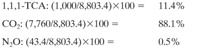
Discussion: This case study demonstrates that the majority of the global warming impact from the production of 1,1,1-TCA is from the energy requirement of the process and not from the emission of the chemical with the highest global warming potential. This analysis assumes that a fossil fuel was used to satisfy the energy requirements of the process. If renewable resources were used (biomass-based fuels), the impact of CO₂ on global warming would be significantly reduced. Finally, the majority of the global warming impact of 1,1,1-TCA could very well be felt during the use stage of its life cycle, not the production stage. A complete life cycle assessment (see Chapter 13) of 1,1,1-TCA is necessary to demonstrate this.

11.3.2 Ozone Depletion

The ozone depletion potential (ODP) of a chemical is the predicted time- and height-integrated change δ[O₃] in stratospheric ozone caused by the release of a specific quantity of the chemical relative to that caused by the same quantity of a benchmark compound, trichlorofluoromethane (CFC-11, CCl₃F) (Fisher et al., 1990b).

Model calculations for ODP have been carried out using one- and twodimensional photochemical models. A list of ODPs for a small number of chemicals has been assembled by a committee of experts (WMO, 1990b and 1992b) and have appeared on separate lists (Heijungs et al., 1992; Goedkoop, 1995). The product of the ODP and the mass emission rate of a chemical i results in the equivalent impact of an emission of CFC-11. Appendix D, Table D-2 hows a list of ozone depletion potential values for important industrial compounds. Data on the tropospheric reaction lifetimes (τ), stratospheric atomic oxygen reaction rate constant (k), and number of chlorines in each molecule (X) are also listed. Notice that the brominated compounds in this table have much larger ODPs than the chlorinated species. Also, it is thought that fluorine does not contribute to ozone depletion (Ravishankara, et al., 1994). Like the global warming chemicals in Appendix D Table D-1, the chemicals in Appendix D, Table D-2 will exist almost exclusively in the atmosphere after being emitted by sources. The ozone depletion index for an entire chemical process is the sum of all contributions from emitted chemicals multiplied by their emission rates. The equivalent emission of CFC-11 for the entire process is then;

11.3.3 Acid Rain

The potential for acidification for any compound is related to the number of moles of H⁺ created per number of moles of the compound emitted. The balanced chemical equation can provide this relationship;

where X is the emitted chemical substance that initiates acidification and α(moles H⁺/mole X) is a molar stoichiometric coefficient. Acidification is normally expressed on a mass basis and therefore the H⁺ created per mass of substance emitted (η_i, moles H⁺/kg i) is:

where MW_i is the molecular weight of the emitted substance (moles i/kg i). As before, we can introduce a benchmark compound (SO₂) and express the acid rain potential (ARP_i) of any emitted acid-forming chemical relative to it (Heijungs et al., 1992):

The number of acidifying compounds emitted by industrial sources is limited to a rather small number of combustion byproducts and other precursor or acidic species emitted directly onto the environment. Appendix D, Table D-3 lists the acid rain potentials for several common industrial pollutants. The total acidification potential of an entire chemical process is defined similarly to I_GW and I_OD.

11.3.4 Smog Formation

The most important process for ozone formation in the lower atmosphere is photodissociation of NO₂:

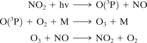
where M is nitrogen or molecular oxygen. This cycle results in O₃ concentration being in a photostationary state dictated by the NO₂ photolysis rate and ratio of [NO₂]/[NO]. The role of VOCs in smog formation is to form radicals which convert NO to NO₂ without causing O₃ destruction, thereby increasing the ratio [NO₂]/[NO], and increasing O₃.

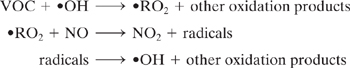
The tendency of individual VOCs to influence O³ levels depends upon its hydroxyl radical (•OH) rate constant and elements of its reaction mechanism, including radical initiation, radical termination, and reactions which remove NOx. Simplified smog formation potential indexes have been proposed based only on VOC hydroxyl radical rate constants, but these have not correlated well with model predictions of photochemical smog formation (Allen, et al., 1992; Japar, et al., 1991).

Incremental reactivity (IR) has been proposed as a method for evaluatingsmog formation potential for individual organic compounds. It is defined as the change in moles of ozone formed as a result of emission into an air shed of one mole (on a carbon atom basis) of the VOC (Carter and Atkinson, 1989). Several computer models have been developed to evaluate incremental reactivity (Bufalini and Dodge, 1983; Carter and Atkinson, 1989; Carter, 1994; Chang and Rudy, 1990; Dodge, 1984). In general, predicted VOC incremental reactivities are greatest when NOx levels are high relative to reactive organic gases (ROG) and lowest (or even negative) when NOx is relatively low. Therefore, the ratio ROG/NOx is an important model parameter. Lists of incremental smog formation reactivities for many VOCs have been compiled (Carter, 1994; Heijungs et al., 1992). An estimation methodology has also been developed which circumvents the need for computer model predictions, though the practical use of this method is limited due to lack of detailed smog reaction mechanisms for a large number of compounds (Carter and Atkinson, 1989). Although several reactivity scales are possible, the most relevant for comparing VOCs is the maximum incremental reactivity (MIR), which occurs under high NOx conditions when the highest ozone formation occurs (Carter, 1994).

The smog formation potential (SFP) is based on the maximum incremental reactivity scale of Carter (Carter, 1994):

where MIR_ROG is the average value for background reactive organic gases, the benchmark compound for this index. This normalized and dimensionless index is similar to the one proposed by the Netherlands Agency for the Environment (Hei-jungs et al., 1992). Appendix D, Table D-4 contains a listing of calculated MIR values for many common volatile organic compounds found in fuels, paints, and solvents. Most of the chemicals in Appendix D, Table D-4 are volatile and will maintain a presence in the atmosphere after release into the air, with the exception of the higher molecular weight organics. The total smog formation potential is the sum of the MIRs and emission rates for each smog-forming chemical in the process. The process equivalent emission of ROG is;

Example 11.3-2 Solvent Recovery from a Gaseous Waste Stream: Effect of Process Operation on Indexes for Global Warming, Smog Formation, and Acidification

A gaseous waste stream is generated within a plastic film processing operation from a drying step. The stream (12,000 scfm) is currently being vented to the atmosphere and it contains 0.5% (vol.) of total VOCs having equal mass percentages of toluene and ethyl acetate with the balance being nitrogen. Figure 11.3-1 is a process flow diagram of an absorption technology configuration to recovery and recycle the VOCs back to the film process (Sangwichien, 1998). Since the waste stream may already meet environmental regulations for smog formation and human toxicity, the key issue is how much of the VOCs to recover and how much savings on solvent costs can be realized. In this problem, we do not deal with the economic issues, but rather show that when considering environmental impacts, there are trade-offs for several impacts depending on the percent recovery of the VOCs.

Figure 11.3-1 Schematic diagram (from HYSYS, Hyprotech, Calgary, Canada) of a solvent recovery and recycle process using absorption into heavy oil (n-tetradecane) followed by distillation.

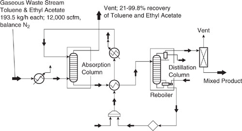
The gaseous waste stream enters the absorption column where the VOCs (toluene and ethyl acetate) transfer from the gas phase to the absorption oil (tetradecane). The effectiveness of this transfer depends largely on the oil flow rate, as the percent recovery of VOCs increases with increasing oil flow rate. The VOCs are sepa-rated from the absorption oil in the distillation column and the oil is then recycled back to the absorption column after cooling. The VOCs are recovered as a mixed product from the condenser of the distillation column and stored in a tank for re-use in the plastic film process. The main emission sources are the absorption column, the vent on the distillation column, the vent on the storage tank (not shown), utility related pollutants, and fugitive sources.

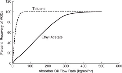
Solution: Table 11.3-2 shows the effect of absorber oil flow rate on the emissions from the solvent recovery process. A commercial process simulator (HYSYS) was used to generate mass and energy balances and to calculate the VOC emission rates from the absorber unit. Within the Environmental Fate and Risk Assessment Tool (EFRAT, ^© refer to Appendix F for a list of software resources.) EPA emission factors and correlations were used to calculate VOC emission rates from the distillation column, storage tank, and fugitive sources. CO₂, CO, TOC, NOx, and SOx emission rates were also calculated within EFRAT based on the energy requirements of the process and an assumed fuel type (fuel oil no. 4). Figure 11.3-2 shows the recovery of toluene and ethyl acetate as a function of absorption oil flow rate in the process. As the absorber oil flow rate is increased, the emissions of toluene and ethyl acetate from the absorber unit decrease, reflecting an increased percent recovery from the gaseous waste stream. Most of the toluene (99.5%) is recovered at a flow rate of only 50 kg-moles/hr. To recover a significant percentage of ethyl acetate requires a much larger oil flow rate. Toluene is recovered more quickly with oil flow rate compared to ethyl acetate because the oil is more selective towards toluene. Emissions of the utility-related pollutants (CO₂, CO, TOC, NOx, and SOx) increase in proportion to the oil flow rate. The emissions of the absorption oil (n-C14) remains relatively constant with oil flow rate.

Table 11.3-2 Air Emission Rates of Chemicals From the Solvent Recovery Process of Figure 11.3-1 (Adapted from Hiew, 1998).

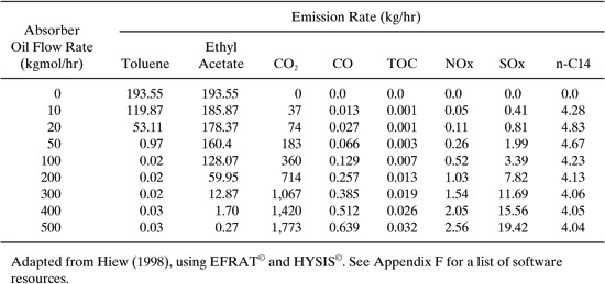
Figure 11.3-2 VOC recovery efficiency for the solvent recovery process of Figure 11.3-1. Adapted from Hiew (1998) and Shonnard and Hiew (2000).

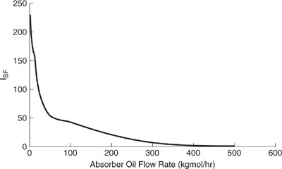
Relative risk indexes for global warming, smog formation, and acidification have been calculated for the solvent recovery process at each flow rate. These values were generated by applying Equations 11-4, 11-13 and 11-11, respectively,

using the emission rates in Table 11.3-2 and the impact potential values for each chemical (Appendix D, Table D-1, D-3, and D-4). For the smog formation potential (SFP = MIR) of ethyl acetate, the average MIR of the ethers (1.13) and ketones (0.87) listed in Appendix D, Table D-4 were used as an approximation. As an example calculation, the smog formation index of the process will be determined at an absorption oil flow rate of 50 kgmole/hr.

Shown in Figures 11.3-3 through 11.3-5 are the relative impact indexes for the sol-vent recovery process of Figure 11.3-1. We observe in Figure 11.3-3 that the global warming index is minimized by operating the process at approximately 50 kgmole/hr. An explanation for this behavior follows next. At an oil flow rate of 0 kgmole/hr, all of the VOCs are emitted directly to the air, resulting in an elevated global warming impact after the organics are oxidized to CO₂. Nearly a 40% reduction in the global warming index is realized by operating the process at an absorption oil flow rate of 50 kgmole/hr. However, above 50 kgmole/hr, the process utilities increase at a substantial rate compared to the rate of additional recovery of the VOCs, driving the index higher. Therefore, the optimum flow rate is approximately 50 kgmole/hr for global warming. As shown in Figure 11.3-4, the acid rain index for the process increases in nearly direct proportion to the absorption oil flow rate. This behavior occurs because the only acidifying species emitted from the process are from the process utility requirements (SOx and NOx), which increase in proportion to the absorption oil flow rate. The optimum flow rate for acidification would be at 0 kgmole/hr for the absorption oil flow rate. The smog formation index (Figure 11.3-5) shows a significant decrease in the index with absorption oil flow rate up to 50 kgmole/hr (recovery of toluene) and a gradual decrease from 50 to 500 kgmole/hr (recovery of ethyl acetate). The flow rate for minimizing the smog formation index is therefore about 500 kgmole/hr.

Figure 11.3-3 The global warming index for the solvent recovery process of Figure 11.3-1. Adapted from Hiew (1998) and Shonnard and Hiew (2000).

Figure 11.3-4 The acid rain index for the solvent recovery process of Figure 11.3-1. Adapted from Hiew (1998) and Shonnard and Hiew (2000).

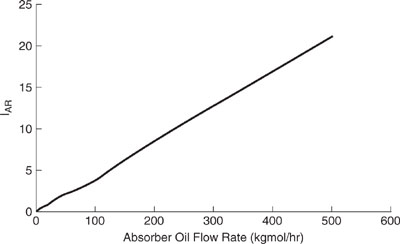
Discussion: These indexes demonstrate the complexities in evaluating chemical processes using multiple indexes of environmental performance. It is not possible to identify a single absorption oil flow rate that simultaneously minimizes all three indexes. However, we can see that significant reductions in the global warming (42%) and the smog formation (82%) indexes are realized at an oil flow rate of 50 kgmole/hr, with only a relatively modest increase in the acid rain index. This observation suggests that a decision to operate the process at 50 kgmole/hr is a good compromise. In reality, the decision to operate the process at any given flow rate will only be made after economic and safety considerations have been taken into account.

Figure 11.3-5 The smog formation index for the solvent recovery process of Figure 11.3-1. Adapted from Hiew (1998) and Shonnard and Hiew (2000).

11.3.5 Toxicity

As explained in Chapter 2, chemical toxicity to humans and ecosystems is a function of dose and response. The dose is dependent on a complex series of steps involving the manner of release, environmental fate and transport of chemicals, and uptake mechanisms. The final two steps dictate the extent of exposure. Key questions which affect the administered dose include: Where are the emissions released to—the air, water, or soil? Are the chemicals altered by environmental reactions or are the chemicals persistent? How are the chemicals taken up by the body? Through breathing contaminated air? Drinking contaminated water? By direct contact with and transfer through the skin? The effective dose is dependent on processes occurring in the body including absorption, distribution, storage, transformation, and elimination. The response by the target organ in the body is a very complex function of chemical structure and modes of action and is the purview of the field of toxicology.

Clearly, the complexity of toxicology precludes an exact determination of all adverse effects to human and ecosystem health from the release of a chemical. From an engineering point of view, an exact assessment may not be necessary. Similar to the potential impact indexes presented for global warming, stratospheric ozone depletion, smog formation, and acidification, we develop and use toxicity potentials for non-carcinogenic and carcinogenic health effects for ingestion and inhalation routes of exposure. Both inhalation and ingestion are thought to be the dominant routes of exposure for human contact with toxic chemicals in the environment.

Non-Carcinogenic Tox

Non-carcinogenic toxicity in humans is thought to be controlled by a threshold exposure, such that doses below a threshold value do not manifest a toxic response whereas doses above this level do. A key parameter for each chemical is therefore its reference dose (RfD (mg/kg/d) or reference concentration (RfC (mg/m³)) for ingestion and inhalation exposure, respectively. Exposures to concentrations in the water or air which result in doses or concentrations above these reference levels is believed to cause adverse effects. Lists of RfD and RfC data are available in electronic or paper copy form (US EPA, 1997; US EPA, 1994). Because RfDs and RfCs are not available for all chemicals, we use lethal doses (LD₅₀) and concentrations (LC₅₀) as additional toxicological parameters for health assessments. Lists of LD₅₀ and LC ₅₀ are tabulated in additional sources (NTP, 1997). Threshold Limit Values (TLVs), Permissible Exposure Limits (PELs), and Recommended Exposure Limits (RELs) are additional toxicity properties that, like RfD and RfC, are based on low-dose studies.

For the purpose of an approximate assessment of risk, concentrations in the air or water will be calculated using the multimedia compartment model shown in Section 11.2. The toxicity potential for ingestion route exposure is defined in this text as:

C_i,w and C_Toluene,w are the steady-state concentrations of the chemical and the benchmark compound (toluene) in the water compartment after release of 1000 kg/hr of each into the water compartment, as predicted by the multimedia compartment model of Section 11.2. The factor of 2 L/d and 70 kg are the standard ingestion rate and body weight used for risk assessment (Pratt, et al., 1993). The product of the concentration and the ingestion rate divided by the body weight provides the exposure dose. This exposure dose is divided by the reference dose to determine whether this dose poses a toxicological risk. The ratio of these risks for the chemical and the benchmark compound results in the ingestion toxicology potential for chemical i.

The toxicity potential for inhalation exposure is defined similarly as:

where C_i,a and C_Toluene,a are the concentrations of chemical i and of the benchmark compound (toluene) in the air compartment of the environment after release of 1000 kg/hr of each into the air compartment, as predicted by the multimedia compartment model. The doses are not shown in the equation because the inhalation rate (20 m³/d) and body weights (70 kg) cancel out. In this equation, the ratio of the risks for inhalation exposure is the potential for inhalation toxicity relative to the benchmark compound.

In order to determine a non-carcinogenic toxicity index for the entire process, we must multiply each chemical’s toxicity potential with its emission rate from the process and sum these for all chemicals released.

Similarly for inhalation route toxicity;

Carcinogenic Toxicity

In a similar method as outlined for non-carcinogenic toxicity, we develop two indexes for cancer-related risk, based on predicted concentrations of chemicals in the air and water from a release of 1000 kg/hr. The concentrations are converted to doses using standard factors and then the risk for the chemical and a benchmark compound, benzene, is calculated. The carcinogenic potential for a chemical is determined by taking the ratio of the chemical’s risk to that for the benchmark compound. The ingestion route carcinogenic potential for a chemical is:

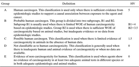
where SF (mg/kg/d)^-1, the cancer potency slope factor, is the slope of the excess cancer versus administered dose data. The dose-response data is normally taken using animal experiments and extrapolated to low doses. The higher the value of SF, the higher is the carcinogenic potency of a chemical. Lists of SF values for many chemicals can be found in the following references (US EPA, 1997; US EPA, 1994). Because SFs are not yet available for all chemicals of interest, weight of evidence (WOE) classifications have been tabulated for many industrial chemicals by consideration of evidence by a panel of experts. The definitions of each weight of evidence classification is shown in Table 11.3-3 along with a numerical hazard value (HV). The value of HV can be used in Equations 11-18 and 11-19 in the absence of SF data. Data for WOE can be found in the following sources (NIHS, 1997; OSHA, 1997; IRIS, 1997).

A similar definition for the inhalation carcinogenic potential for a chemical is:

The carcinogenic toxicity index for the entire process is again a summation for each carcinogen. For ingestion, it is:

and for inhalation,

Example 11.3-3 Toxicity Evaluation of the Solvent Recovery Process in Figure 11.3-1

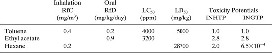
Toxicity evaluation of the toluene and ethyl acetate recovery and recycle process design is conducted in a fashion similar to the previous example problem. We are concerned with three compounds in this analysis, toluene, ethyl acetate, and hexane (a surrogate for products of incomplete combustion in utility consumption). There are no carcinogenic compounds present in the design, therefore the two carcinogenic indexes will be ignored. This example illustrates how LD₅₀/LC₅₀ can be used interchangeably with RfDs and RfCs when data gaps occur.

Data and Results: The emission rates of these compounds appeared in the previous example problem and are used again here. The concentrations of these chemicals and the benchmark compound (toluene again) are calculated using the Mackay model of Section 11.2. The input data and the resulting concentrations are provided in the following table. The calculations were conducted using a standard emission of 1000 kg/hr of each compound into the air compartment when evaluating both ingestion toxicity and inhalation toxicity. This approach was adopted rather than using the actual emission rates of each compound, because only the ratios of concentrations are needed in the index calculation, and the concentration ratios are not a function of emission rate using the Mackay model.

Table 11.3-3 Weight of Evidence (WOE) Classifications (IRIS, 1997; Davis et al., 1994).

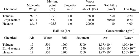
The toxicological properties (RfDs, RfCs) are incomplete for the three chemicals in this design. We are forced to use LD₅₀ and LC₅₀ data when gaps occur. The following table summarizes the toxicology data and calculated ingestion and inhalation toxicity potentials using the air and water concentrations in the table above and the toxicity Equations 11-14 and 11-15.

Figures 11.3-6 and 11.3-7 show the change in process inhalation and ingestion toxicity index with absorption oil flow rate using the emission rate data tabulated in the previous example problem and concentrations calculated by the Mackay model.

Discussion: The inhalation toxicity is reduced with increasing absorption oil flow rate due to the removal of both toluene and ethyl acetate, and to a much lesser extent by hexane (TOC). The inhalation and ingestion index behavior is nearly identical since the inherent toxicity potentials, INHTP and INGTP, are virtually the same (as shown above). These toxicity indexes can be reduced by 39% by operating the process at 50 kgmoles/hr absorber flow rate. Keep in mind that interchanging RfCs with LC₅₀s will introduce additional uncertainties in the evaluation.

Summary

This chapter has outlined a systematic methodology for evaluating environmental and health-based impacts for chemical process designs. Multiple impact indexes are included for process evaluation because of the complexity of pollutant interactions with the environment and with human health. The methodology includes pollutant release or emission estimation (Chapter 8), environmental fate and transport of pollutants, and relative risk assessment using the benchmarking concept. The methodology was applied for the evaluation of air emissions from a process flowsheet utilizing a commercial chemical process simulator to generate the material and energy balances for the process. From this analysis, we were able to assess the environmental performance of the process as one of the process parameters, the absorber oil flow rate, was varied over a wide range. This exercise provided insights into how energy consumption within the process drives up certain environmental impacts and how the recovery and recycle of VOCs drives down others. The trends for impact with respect to absorber oil flow rate are clear, but making a decision based on these trends is not straightforward. Since trade-offs do occur among these impact indexes, questions such as which impacts are most important need to be addressed. Nonetheless, the environmental information provided will allow for more sound process design decisions.

Figure 11.3-6 Inhalation toxicity index for the solvent recovery and recycle process.

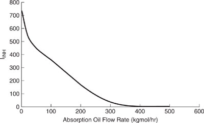
Figure 11.3-7 Ingestion toxicity index for the solvent recovery and recycle process.

It is important to stress that the methodology is general, and can accommodate releases to the water and the soil as well as to the air, since the multimedia compartment model can predict environmental concentrations for all of these release mechanisms. Another issue to consider is the uncertainties involved in the assessment of environmental risk. There are many sources of uncertainty, particularly for emission estimation and environmental fate calculations. The magnitude of these uncertainties may be quite large, depending upon the emission estimation method and on chemical-specific environmental properties. It is important to understand the magnitude of these uncertainties in order to decide whether significant differences actually occur when comparing the environmental impacts of process operating conditions or of various process technologies. Uncertainty analysis for environmental impact assessment is an active research area in chemical engineering and in environmental science and engineering. The topic is beyond the scope of this introductory textbook, but methods of evaluating uncertainty are available, and may include Monte Carlo simulation and propagation of error analysis.

References

Allen, D.T., Bakshani, N., and Rosselot, K.S., “Pollution Prevention: Homework & Design Problems for Engineering Curricula,” American Institute of Chemical Engineers, New York, NY, 155 pages, 1992.

Allen, D.T. and Rosselot, K.S. “Pollution Prevention for Chemical Processes,” 1st ed., John Wiley & Sons, New York, NY, 434 pages, 1997.

Bufalini, J. J. and Dodge, M. C. “Ozone-forming potential of light saturated hydrocarbons,” Environmental Science and Technology 1983, 17, 308.

Boustead, I., “Ecoprofiles of the European Plastics Industry, Report 1–4,” PQMI, European Centre for Plastics in the Environment, Brussels, May, 1993.

Carter, W. P. and Atkinson, R. “A computer modeling study of incremental hydrocarbon reactivity,” Environmental Science and Technology 1989, 23, 864–880.

Carter, W. P. L., “Development of ozone reactivity scales for volatile organic compounds,” Air & Waste 1994, 44, 881–899.

Chang, T. Y. and Rudy, S. J., “Ozone-forming potential of organic emissions from alternative-fueled vehicles,” Atmospheric Environment 1990, 24A, 2421.

Cohen, Y., Tsia, W., Chetty, S. L. and Mayer, G. J., “Dynamic partitioning of organic chemicals in regional environments: A multimedia screening-level modeling approach,” Environ. Sci. Technol. 1990, 24, 1549–1558.

Davis, G.A., Kincaid, L., Swanson, M., Schultz, T., Bartmess, J., Griffith, B., and Jones, S., “Chemical Hazard Evaluation for Management Strategies: A Method for Ranking and Scoring Chemicals by Potential Human Health and Environmental Impacts,” United States Environmental Protection Agency, EPA/600/R-94/177, September 1994.

Derwent, R.G., “Trace Gases and Their Relative Contribution to the Greenhouse Effect,” Atomic Energy Research Establishment, Report AERE-R13716, Harwell, Oxon, 1990.

Dodge, M. C., “Combined effects of organic reactivity and NMHC/NOx ratio on photochemical oxidant formation—a modeling study,” Atmospheric Environment 1984, 18, 1857.

Fetter, C.W., Contaminant Hydrogeology, Prentice-Hall, Inc., pg. 458, 1993.

Fisher, D.A., Hales, C.H., Wang, W., Ko, M.K.W., and Sze, N.D., “Model calculations of the relative effects of CFCs and their replacements on global warming,” Nature, vol. 344, 513–516, 1990a.

Fisher, D.A., Hales, C.H., Filkin, D.L., Ko, M.K.W., Sze, N.D., Connell, P.S., Wuebbles, D.J., Isaksen, I.S.A., and Stordal, F., “Model calculations of the relative effects of CFCs and their replacements on stratospheric ozone,” Nature, Vol. 344, 508–512, 1990b.

Goedkoop, M., “The Eco-indicator 95, Final Report,” Netherlands Agency for Energy and the Environment (NOVEM) and the National Institute of Public Health and Environmental Protection (RIVM), NOH report 9523, 1995

Heijungs, R., Guinée, J.B., Huppes, G., Lankreijer, R.M., Udo de Haes, H.A., Sleeswijk, A. Wegener, “Environmental Life Cycle Assessment of Products. Guide and Backgrounds,” NOH Report Numbers 9266 and 9267, Netherlands Agency for Energy and the Environment (Novem), 1992.

Hiew, D.S., “Development of the Environmental Fate and Risk Assessment Tool (EFRAT) and Application to Solvent Recovery from a Gaseous Waste Stream,” Masters Thesis, Department of Chemical Engineering, Michigan Technological University, 1998.

IPCC, “Radiative Forcing of Climate, Climate Change—The IPCC Scientific Assessment: 1990 (WMO),” Cambridge University Press, 45–68, 1991.

IPCC, “Climate Change 1994—Radiative Forcing of Climate Change and an Evaluation of the IPCC IS92 Emission Scenarios,” Intergovernmental Panel on Climate Change, J.T. Houghton et al. (ed.), Cambridge University Press, 1994.

IPCC, “Climate Change 1995—The Science of Climate Change,” Intergovernmental Panel on Climate Change, J.T. Houghton et al. (ed.), Cambridge University Press, 1996.

IRIS, Integrated Risk Information System (IRIS), http://www.epa.gov/ngispgm3/iris/Substance_List.html, US Environmental Protection Agency, 7/15/97.

Japar, S. M., Wallington, T. J., Rudy, S. J., and Chang, T. Y., “Ozone-forming potential of a series of oxygenated organic compounds,” Environmental Science and Technology 1991, 25, 415–420.

Lashof, D.A. and Ahuja, D.R., “Relative contributions of greenhouse gas emissions to global warming,” Nature, Vol. 344, 529–531, 1990.

Mackay, D. Multimedia Environmental Models, The Fugacity Approach Second Edition, CRC Press 2001; pg. 272.

Mackay, D, and Paterson, S., “Evaluating the multimedia fate of organic chemicals: A level III fugacity model,” Environmental Science and Technology, V. 25 (3), pg 427–436, 1991.

Mackay, D., Shiu, W., and Ma, K., Illustrated Handbook of Physical-Chemical Properties and Environmental Fate for Organic Chemicals, 1st edition, Vol. 1–4, Lewis Publishers, Chelsea, MI, 1992.

Mallick, S.K., Cabezas, H., Bare, J.C., and Sikdar, S.K., “A pollution reduction methodology for chemical process simulators,” Industrial & Engineering Chemistry Research, Vol. 35, (11), 4128-, 1996.

McKone, T. E., 1994, “CALTOX, A Multimedia Total Exposure Model for Hazardous Waste Sites,” Version 1.5, IBM/PC, Microsoft Excel Spreadsheet Program, National Technical Information Service, Springfield, VA, Order No. PB95-100467.

NRC (National Research Council), “Risk Assessment in the Federal Government: Managing the Process,” Committee on Institutional Means for Assessment of Risks to Public Health, National Academy Press, Washington, D.C. (1983).

NTP, National Toxicology Program, Chemical Health & Safety Data, http://ntp-db.niehs. nih.gov/Main_pages/Chem-HS.HTML, 7/15/97.

OSHA, Occupational Safety & Health Administration, http://www.osha-slc.gov/ChemSamp_toc/ChemSamp_toc_by_chn.html Chemical Sampling Information, Table of Contents by Chemical Name, U.S. Department of Labor, 7/15/97.

Pouchert, C.J., “The Aldrich Library of FT-IR Spectra, Vapor Phase,” 1st edition, Vol. 2, pg. 165–229, 1989.

Pratt, G.C., Gerbec, P.R., Livingston, S.K., Oliaei, F., Bollweg, G.L., Paterson, S., and Mackay, D., “An indexing system for comparing toxic air pollutants based upon their potential environmental impacts,” Chemosphere, Vol. 27 (8), 1359–1379, 1993.

Ravishankara, A.R., Turnipseed, A.A., Jensen, N.R., Barone, S., Mills, M., Howard, C.J., and Solomon, S., “Do hydrofluorocarbons destroy stratospheric ozone?,” Science, Vol. 263, 71–75, 1994.

Rotmans, J.; “IMAGE, an Integrated Model to Assess the Greenhouse Effect,” Maastrich, pp 205–224, 1990.

Sangwichien, C., “Modeling and Evaluating Solvent Recovery Technologies Applied to Industrial Pollution Prevention,” Masters Thesis, Department of Chemical Engineering, Michigan Technological University, 1998.

Seinfeld, J.H. and Pandis, S., “Atmospheric Chemistry and Physics: Air Pollution to Climate Change,” John Wiley & Sons, New York, NY, pg 1326, 1997.

SETAC, Society for Environmental Toxicology and Chemistry, “Guidelines for Life-Cycle Assessment: Code of Practice,” Brussels, Belgium, 1993.

Shonnard, D.R. and Hiew, D.S., “Comparative Environmental Assessments of VOC Recovery and Recycle Design Alternatives for a Gaseous Waste Stream,” Environmental Science and Technology, 34(24), 5222–5228, 2000.

Thibodeaux, L.J., Environmental Chemodynamics, Second Edition, John Wiley & Sons, New York, NY, pg 593, 1996.

US EPA, Health Effects Assessment Summary Tables (HEAST), 1994.

US EPA, Integrated Risk Information System (IRIS), 1997.

US EPA, Locating and Estimating Air Emissions From Sources, U.S. Environmental Protection Agency, Air CHIEF, Version 8.0, Office of Air Quality Planning and Standards, EPA 454/C-00–003 December 2000.

WMO, “Halocarbon Ozone Depletion and Global Warming Potential, Scientific Assessment of Stratospheric Ozone: 1989,” World Meteorological Organization, Report number 20, Vol. 1, 1990a.

WMO, “Executive Summary: Supporting Evidence and Other Results, Scientific Assessment of Stratospheric Ozone: 1989,” World Meteorological Organization, Report number 20, Vol. 1, 1990b.

WMO, “Radiative Forcing of Climate, Scientific Assessment of Global Warming: 1991,” World Meteorological Organization, Report number 25, Vol. 1, 1992a.

WMO, “Ozone Depletion and Chlorine Loading Potential, Scientific Assessment of Ozone Depletion: 1991,” Global Ozone Research and Monitoring Project, World Meteorological Organization, Report number 25, Vol. 1, 1992b.

Problems

1. Ethanol as a Substitute Octane-Boosting Additive to Automobile Fuels. In response to requirements of the 1990 Clean Air Act Amendments, automobile fuels sold in some urban areas must contain 10% ethanol. The reasons for adding ethanol are 1) to reduce emissions of carbon monoxide from tail pipes, and 2) to boost the octane rating of the resulting fuel blend. The maximum incremental reactivity (MIR) values for ethanol and other potential octane boosters are provided below.

Ethanol 1.34

Toluene 2.70

Xylenes 7.10

Base Fuel 1.5

Calculate by what percentage the ozone-producing potential of an ethanol fuel blend (10% ethanol, 90% base fuel) is reduced compared to a fuel blend containing 10% toluene and 90% base fuel and another blend containing 10% xylenes and 90% base fuel, respectively. Use the provided MIR values in Appendix D, Table D-4 for this calculation and assume that the MIR of the blend is a summation of each components MIR weighted by its fraction in the blend.

(For a comprehensive discussion of the use of ethanol as a fuel blending component, see National Research Council, “Ozone-forming Potential of Reformulated Gasoline,” National Academy Press, Washington, D.C., 1999)

2. Hydroxyl Radical and Reaction with Ethene. The second-order rate constant for the reaction of ethene with OH• is approximately k = 2.7 × 10^-13 (cm³ / (molecule • sec)). The expression for the rate of reaction of ethene is

Rate = k [OH•] [Ethene]

If [OH•] is maintained at 10^-12 moles per liter in a test chamber, and the initial ethene concentration is 100 ppm, estimate:

a) the pseudo first-order rate constant (k [OH•]) for ethene under these conditions.

b) the amount of ethene remaining after 1 hour

Hint: convert [OH•] from moles per liter of air to molecules per cm³ first before answering part a.

3. Global Warming Parameters. The most important chemical parameters which affect the global warming potential of a greenhouse gas are the reaction lifetime (τ) and the infrared absorbence band strength (BI). Demonstrate the importance of these parameters by performing the following tasks.

a) From Appendix D, Table D-1, group chemicals having the highest values of both and BI and determine whether these have the highest values of GWP.

b) Determine the sensitivity of GWP to τ and BI. Assume that GWP is a continuous function of τ and BI. We can write a change in GWP (dGWP) as functions of changes in (dτ) and BI (dBI) as follows;

where (∂GWP/∂τ)_BI is the partial derivative of GWP with respect to τ holding BI constant. The other partial derivative is similarly defined. Estimate the partial derivatives for GWP using the data listed in Appendix D, Table D-1.

c) Estimate each term on the right hand side of the equation above by using dτ = 10 years and dBI as 400 atm^-1 cm^-2. Which term contributes the most to changes in GWP (d(GWP))?

4. Incremental Reactivities of Volatile Organic Compounds. Appendix D, Table D-4 shows maximum incremental reactivities (MIR) for many volatile organic compounds found in urban areas. Use entries from the first column of data in this table to answer the following questions.

a) How do the averages for each of the classes of compounds compare to the average for the entire list (Base ROG Mixture)?

b) If you were in charge of reformulating a fuel for automobiles, what class of compounds would you retain for a more detailed consideration as a substitute fuel component if one of the main considerations is reducing smog formation potential? Based on this analysis, why has ethanol been used as a substitute? What other considerations (environmental and non-environmental) have to be taken into account in choosing a compound to add to make a reformulated gasoline?

5. Environmental Risk Index Calculations for Solvent Recovery and Recycle. Calculate and then compare the environmental and human health indexes for the solvent recovery process shown in Example 11.3-2 for absorber oil flow rates of 0 and 100 kgmoles/hr. Use the emission rate data shown in Table 11.3-2 of Example 11.3-2 and use hexane as a surrogate (representative compound) for TOC. In your analysis, calculate the indirect global warming potential for each VOC. Assume that Fuel Oil #4 is being used to satisfy the energy demand of the processes and that this fuel contains 1% sulfur. Use the RfD, RfC, LD₅₀, and LC₅₀ values and employ the multimedia concentrations of each component in the air and water as shown in Example 11.3-3.

6. Carbon Dioxide Emission Factors (Chapter 8). Confirm the CO₂ emission factors listed in the text (Tables 8.3-5 and 8.3-6) for fuel oil and natural gas. As an approximation, assume that fuel oil is composed entirely of n-decane (C₁₀H₂₂) and that natural gas is 100% methane (CH₄). Use the ideal gas law and standard conditions of 0°C and 1 atmosphere pressure for the natural gas calculation. The specific gravity of n-decane is 0.73. The reaction stoichiometries for the combustion reactions are:

C₁₀H₂₂ + 15 1/2 O₂ → 10CO₂ + 11 H₂O

CH₁₀ + 2 O₂ → CO₂ + 2 H₂O