
2.6. SLITTING (CRACK COMPLIANCE) METHOD 25
like wood whose physical properties are highly variable and typically are not accurately known
without further testing.
Figure 2.3c shows another geometrical variant of the Splitting Method, commonly used
to assess the circumferential residual stresses in thin-walled heat exchanger tubes. Diameter
increase caused by the opening of the cut indicates tensile circumferential stresses around the
exterior surface of the tube, balanced by compressive stresses around the interior. Diameter de-
crease indicates the opposite. e experimental method is well-established and is specified by
ASTM Standard Test Procedure E1928. e approximate sizes of the surface circumferential
stresses can be estimated using:
D ˙
Et
1
2
D D
0
DD
0
; (2.1)
where
are the circumferential bending stresses at the outer (C) and inner () surfaces, D
0
and D, respectively, are the diameters before and after making the cut, t is the wall thickness,
E is Young’s modulus and is Poisson’s ratio. e calculated results are approximate because
Equation (2.1) is based on an assumption of linearly varying bending stresses through the tube
wall thickness. In practice, the residual stresses do not vary exactly linearly.
2.6 SLITTING (CRACK COMPLIANCE) METHOD
From a conceptual point of view, the Slitting Method, schematically illustrated in Figure 2.4, is
a further variant of the Two-Groove Method. In this case, relieved strain measurements are
sequentially made as slot cutting proceeds in a series of small incremental steps. e set of
strain measurements provides sufficient data for the evaluation of the stress profile within the
slot depth. is process differs from the typical Two-Groove measurement, where just a single
before-and-after strain measurement is made while cutting the slots in just one step directly to
the steady-state depth. is latter measurement gives only the weighted average stress within
the cut depth, with no within-depth profile information.
e purpose of using two deep slots in the Two-Groove Method is to create full strain
relief in the enclosed material, thereby providing a simple residual stress evaluation. Since a
stress profile measurement using intermediate slot depths involves measurement and analysis
of partial strain reliefs, full strain relief never occurs except perhaps at the very end. us, the
second slot does not provide any computational advantage and so is omitted to simplify the
required experimental procedure. In addition, as shown in Figure 2.4, the strain gauge position
is not limited to being on the specimen top surface. Other locations are also useful, notably on
the opposite surface of the material specimen. As a general rule-of-thumb, strain measurements
are most sensitive to nearby stresses. us, the top and bottom surface strain gauges shown in
Figure 2.4 are useful for determining stresses near their respective locations, thereby achieving
better spatial coverage.

26 2. RELAXATION TYPE RESIDUAL STRESS MEASUREMENT METHODS
Surface Strain Gauge
Back Strain Gauge
Figure 2.4: Slitting Method for measuring residual stresses.
Despite its geometrical similarity to the Two-Groove Method, the historical roots of the
Slitting Method have a separate origin based on an earlier analogy with the strain field around
a crack. e crack analogy provided the needed computational procedure to enable evaluation
of the within-depth stress profile from the set of incrementally measured strains. Based on this
approach, the original procedure name was the Crack Compliance Method. However, the stress
computational procedure is now typically based on numerical calibration data from finite ele-
ment calculations, so the crack analogy is no longer needed. Consequently, the name “Slitting
Method” or “Incremental Slitting Method” has come into more common use.
e typical data from the Slitting Method are the set of strain gauge measurements ac-
quired as the depth of the slit is incrementally increased in small steps. e surface strain ".h/
measured when the slit reaches a depth h is the sum of the relaxation effects of all the perpen-
dicular normal stresses at the various depths within the slit depth:
".h/ D
Z
h
0
A.H; h/ .H/ dH; (2.2)
where .H/ is the normal stress existing at depth H from the surface and A.H; h/ is the strain
response from a unit stress existing at depth H within a slit of current depth h. e compliance
function A.H; h/ is typically determined using finite element calculations. e integral on the
right side appears as a consequence of all the residual stresses over the cut surface combining to
produce the measured strains.
Equation (2.2) is mathematically classified as a Volterra equation of the first kind. It is
an “inverse” equation because the quantities to be determined, the stresses, appear on right side
within the integrand, while the known data, the strains, appear on the left. is is the reverse of
the usual “forward” format. e inverse character of Equation (2.2) substantially complicates the
required solution procedure and causes the stress results to be sensitive to the presence of small
2.6. SLITTING (CRACK COMPLIANCE) METHOD 27
strain measurement errors. Sophisticated mathematical procedures are required to get reliable
stress solutions.
e Slitting Method and Equation (2.2) provide a conceptual prototype for the majority
of the relaxation type of residual stress measurement methods. e common features of these
methods are:
1. Deformations, typically strains, are measured at one or more points on the specimen while
the cut surface is deepened into the interior in a series of small steps. ere is a spatial
separation between the measurement location and the associated stresses within the cut
depth. us, the relationship between the residual stresses and the measured strains is
indirect and requires either analytical or numerical “calibration.” is feature is represented
in Equation (2.2) by the compliance function A.H; h/ also called the “kernel” function.
2. e out-of-plane residual stresses that originally existed along the cut surface within the
cut depth all contribute to the measured strains. Because many stresses contribute to each
measured strain, there is not a one-to-one relationship between individual strains and
stresses. is feature is represented in Equation (2.2) by the presence of the integral on
the right side.
3. e measured strain is mostly controlled by the residual stresses nearest to the measure-
ment location. In mathematical terms, the measured strain response is a weighted average
from the stresses that originally existed over the full cut depth, where the weighting is
heavily biased toward the measurement location.
4. When making measurements at the top surface, the measured strain gradually increases
(and then sometimes slightly decreases) as the cut is extended, reaching a steady-state level
when the cut extends far from the strain measurement location. If the residual stresses are
assumed to have uniform variation within the cut depth, measurement of only the steady-
state strain provides a convenient way to determine the uniform residual stress. is is the
procedure typically used with the Two-Groove Method, where the strain measurement
is made after cutting the slots in one step to a depth at least reaching the steady-state
strain value, which approximately corresponds to the slot separation distance. For the Tube
Splitting Method, the equivalent uniform bending stresses are estimated from the tube
diameter change before and after full splitting of the tube.
5. e general format of Equation (2.2) applies to a wide range of relaxation type methods
for measuring residual stresses. e various methods differ substantially in their specimen
and cut geometries, but mathematically, the associated residual stress calculations fit the
format of Equation (2.2), each method with its own specific compliance function A.H; h/.
Some methods may involve measurements of displacements rather than strains, sometimes
also at more than one point. e details of Equation (2.2) then vary accordingly, but the
overall format remains the same. Figure 2.5 shows example contour plots of cumulative
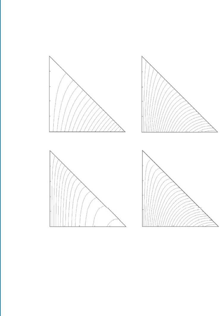
28 2. RELAXATION TYPE RESIDUAL STRESS MEASUREMENT METHODS
compliance functions for several common residual stress measurement methods. Plotted
vertically is the cut depth h, and horizontally the stress depth H . Because only the stresses
within the cut depth can contribute to the strain response, H is always less or equal to h.
is is the reason for the triangular shape of the plots in Figure 2.5 and also for the presence
of h as the upper limit of the integral in Equation (2.2). It can be seen that the various
cumulative compliance functions differ in detail, but have similar overall characteristics.
(a) Sach’s Method (b) Layer Removal
(c) Hole Drilling (d) Slitting
0.0
0.2
0.4
0.6
0.8
1.0
0.0
0.2
0.4
0.6
0.8
1.0
0.0
0.1
0.2
0.3
0.4
0.5
0.0
0.2
0.4
0.6
0.8
1.0
0.0
0.0 0.0
0.0 0.0
0.2
0.2
0.3
0.5
0.7
0.1
0.4
0.4
0.04
0.08
0.12
0.16
0.20
0.24
0.28
0.6
0.6
0.8
0.8
0.9
1.0 0.0 0.2 0.4
0.4
0.6 0.8 1.0
0.8
1.2
1.6
1.6
2.0
2.0
2.4
2.4
0.0 0.1 0.2 0.3 0.4 0.5 0.0 0.2 0.4
0.4
0.6 0.8
0.8
1.0
1.2
Normalized Stress Depth
Normalized Radial Depth
Normalized Layer Depth
Normalized Hole Depth
Normalized Slit Depth
Normalized Stress Depth
Normalized Stress Depth Normalized Stress Depth
Figure 2.5: Cumulative compliance functions for various residual stress measurement methods.
(a) Sachs’ Method, (b) Layer-Removal Method, (c) Hole-Drilling Method, and (d) Slitting
Method (from Schajer and Prime (2006)).
6. A characteristic of an integral equation such as Equation (2.2) is that very different com-
binations of stresses can sum together to produce almost similar corresponding strains.
is characteristic means that small errors in the measured strains can substantially shift
the details of associated stress solution. e mathematical effect is like a “noise amplifier,”
where small noise in the input strain data creates proportionally much larger noise in the
..................Content has been hidden....................
You can't read the all page of ebook, please click here login for view all page.