

152 7. OPTICAL TECHNIQUES
much larger or much smaller than the 0.5–5.0 mm diameter range suited to interferometric
measurements. Figure 7.9 shows examples of such measurements, part (a) showing a 63.5 mm
diameter hole and part (b) showing a 1.5 m diameter hole observed within a scanning electron
microscope.
(a) (b)
Figure 7.9: DIC hole-drilling residual stress measurements at different scales. (a) hole diame-
ter D 63:5 mm (photo from McGinnis et al. (2005)) and (b) hole diameter D 1:5 m (image
courtesy of B. Winiarski).
7.6 COMPUTATION OF UNIFORM RESIDUAL STRESSES
e availability of full-field data from optical measurements presents both opportunities and
challenges. e rich data set provides many possibilities for productive data analysis, for example,
to do data consistency checking and outlier correction, data averaging, evaluation of additional
stress results and measurement artifact compensation. e large size of the data set also creates
challenges as how to handle the substantial bulk of the data in an effective way. Some desired
objectives of a residual stress computation method for use with optical data include to:
• take advantage of the wealth of data available within an optical image;
• extract the data from the image with a minimum of human interaction preferably none;
and
• use the available data in its native form in a compact and stable computation.
7.6. COMPUTATION OF UNIFORM RESIDUAL STRESSES 153
Initial optical measurements for hole-drilling residual stress evaluations used calculation
methods analogous to those for use with strain gauges. Typically, they involved visually pick-
ing a small number of opportune points within the measured images, interpreting their fringe
orders, and then doing a strain gauge style calculation. Such fringe pattern interpretation is an
important need when working with the unsigned analog data that comes from traditional holo-
graphic measurements with photographic or thermoplastic plates. Although effective results are
achieved, the performance of these methods can be further enhanced by including the contri-
butions of the substantial quantity of additional data available beyond the few selected points.
e ESPI, phase-stepped Moiré and DIC methods share the advantage that they provide
signed numerical data. A typical image taken with a modern video camera contains several hun-
dred thousands, often millions of pixels, thus a very large number of independent measurements
are produced. e availability of such large amounts of quantitative data makes these methods
well suited for more in-depth data analysis.
In contrast to the traditional strain gauge style measurements, all optical techniques indi-
cate surface displacements, not strain. Estimation of surface strains from displacement measure-
ments involves numerical differentiation, which is an inherently noisy process, and consequently
is to be avoided. us, it is desirable to choose computation methods that work directly with
displacement data. In addition, linear methods are particularly desirable to achieve effective and
compact data processing. Nonlinear procedures can also be effective, but they are much more
computationally intensive, potentially less stable, and thus should be used only when essential.
A computation that has a greater number of data than unknowns is called “over-
determined.” e number of available optical data is much greater than the number of un-
knowns, so there exists a good opportunity to extract some further results from the measure-
ments. Here, it is very effective also to include in the calculation the effects of systematic artifacts
that can occur in practical experimental measurements. For example, in each of the various op-
tical methods, drifts often occur that cause the data from all image pixels to shift by the same
amount. In the ESPI and Moiré methods such drifts occur from temperature changes within
the apparatus, with DIC they occur from small position changes of the optical components.
Similarly, image stretching can occur due to specimen temperature changes, or to magnification
changes in the case of DIC measurements within a scanning electron microscope. Even with
these additional factors included in the calculation, the residual stress computation is still highly
overdetermined. e excess data can usefully be exploited to provide an averaging effect that
acts to reduce the effect of random measurement noise.
It is generally impossible to achieve a numerical solution of an overdetermined measure-
ment that exactly fits all measured data. Consequently, a “best-fit” solution is sought that is
as close as possible to the majority of the measured data. is can conveniently be done using
the Least-Squares method. is approach was introduced for ESPI measurements by Steinzig
and Ponslet (2003) and further developed by subsequent authors. Figure 7.10 schematically de-
scribes the procedure. e starting point is the measured image shown on the left. is could be
154 7. OPTICAL TECHNIQUES
an unwrapped phase map measured using the ESPI or Moiré methods, or a displacement map
from the DIC method. On the right side are the computed responses to the factors that are
anticipated to contribute to the measurement. In this case, these are the P , Q, and T stresses
and three potential data artifacts. In this single-axis example, where the surface displacements
have been measured in the x-direction only, the artifacts, respectively, are bulk displacement,
uniform stretch and uniform shear, all in the x-direction. For dual axis measurements, the anal-
ogous artifacts in the y-direction could further be included.
≈ w
1
× + w
2
× + w
3
×
+ w
4
× + w
5
× + w
6
×
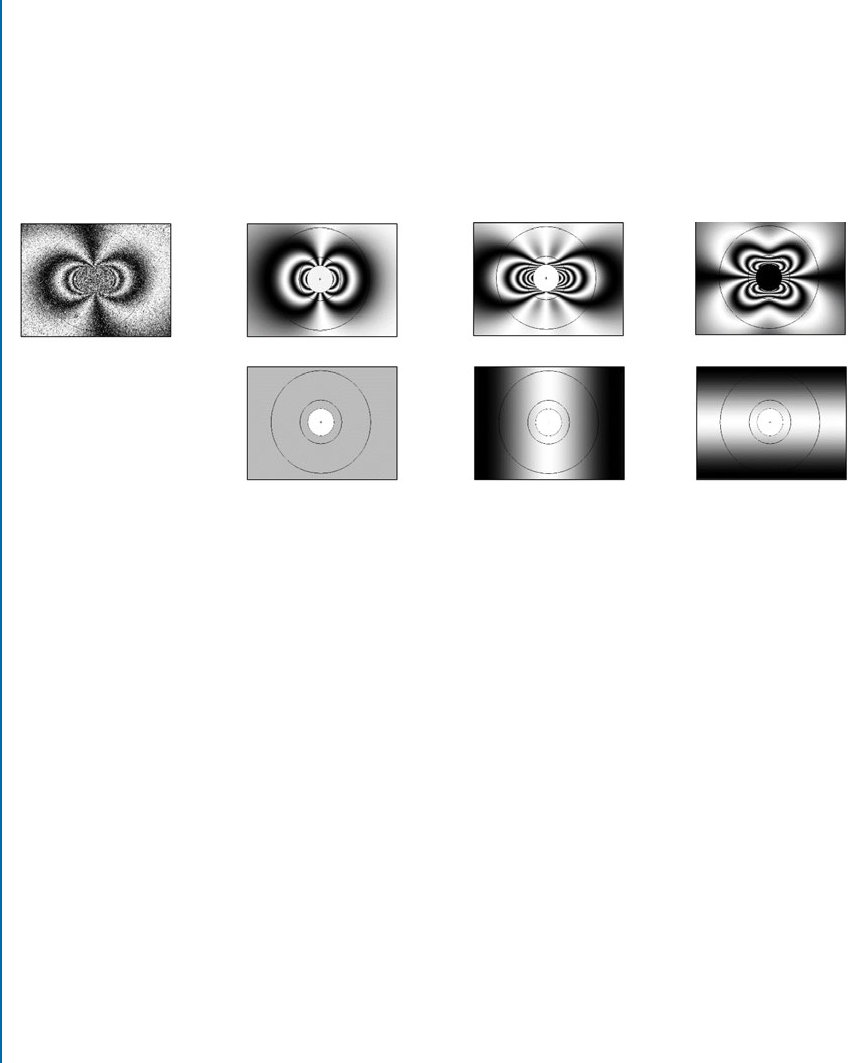
Figure 7.10: Least-squares fit of a measured fringe pattern as a weighted sum of six contribut-
ing factors. 1 D P -stress, 2 D Q-stress, 3 D T -stress, 4 D x-displacement, 5 D x-stretch, and
6 D x-shear.
e six contributing factor images shown in Figure 7.10 represent their individual re-
sponses when each of them has a unit size. e actual sizes of the contributing factors are rep-
resented by the weights w
i
; 1 i 6 that appear as numerical factors. e measured response
on the left can then be interpreted as the weighted sum of the responses on the right, with each
of the right-side source quantities present in the corresponding amounts in the measured speci-
men. e weighting factors w
i
can be determined using the Least-Squares method. It finds the
combination of the weighting factors that gives a sum that most closely fits the measurements
on the left of Figure 7.10.
Figure 7.11 shows the “best-fit” sum of the six contributing factors included in Figure 7.10.
Because of the overdetermination of the calculation, the fit is not exact at every point. e
remaining difference between the measured data and the sum of the best-fit data is called the
“residual.” Ideally, the residual should appear as in Figure 7.11, with uniformly random noise
and without apparent structure.
Practical calculations proceed with the data contained in the images in Figure 7.10 ar-
ranged in vector-matrix format
Gw D ı; (7.1)

7.6. COMPUTATION OF UNIFORM RESIDUAL STRESSES 155
= +
(a) (b) (c)
Figure 7.11: Least-squares fit fringe pattern. (a) Measured fringe pattern, (b) best-fit fringe
pattern, and (c) residual.
where the vector w contains the six weighting factors w
i
. Vector ı contains the displacements
represented by the N pixels in the measured image that are used for the calculation. ese pix-
els are taken from the annular area around the drilled hole shown in the image on the left of
Figure 7.10. is area is chosen to encompass a region that:
• is circular so as to minimize directional bias in the calculation;
• has an inner radius sufficient to exclude pixels damaged by chips scratching the surface as
they exit the drilled hole. However, it should not be so large so as to lose valuable high-
displacement data near the hole edge. In the example in Figure 7.10, the inner radius was
chosen as 1.8 times the hole radius, which excludes most of the damaged pixels visible in
the residual plot, Figure 7.11c; and
• not too distant from the hole so as only to include pixels with significant displacement
data content. Pixels far away from the hole are excluded because the potential benefit of
their displacement data content becomes small compared with the potential damage from
their noise content.
e choice of the inner and outer radii of the selected annular area requires some judgment.
Typical values of the inner radius are between 1.5 and 2.0 times the hole radius. Typical values
of the outer radius are between 3.0 and 4.0 times the hole radius. e latter is not a sensitive
choice and can be selected to fit the scale of the measured image. To facilitate a reasonable
choice, the magnification used for the initial setup of the optical arrangement for a hole drilling
measurement should be set to make the height of the measured image approximately four to five
times the anticipated hole diameter.
Matrix G has N rows corresponding to the pixels in ı and 6 columns corresponding to
the unknowns in w. e contents of the columns are the six unit contributing factors shown on
the right of Figure 7.10, arranged in the same pixel order as in vector ı. Since the three artifacts
represent physically different things from the three stresses, it can happen that the corresponding
156 7. OPTICAL TECHNIQUES
columns of G have elements of greatly differing sizes. is occurrence would seriously impair
the numerical conditioning of the matrix and create significant roundoff error effects. is issue
can be avoided by choosing units for the artifact quantities that give columns in matrix G that
have contents of generally similar size to those in the stress columns.
Since N >> 6, Equation (7.1) is highly overdetermined. e “best-fit” solution can be
determined using the Least-Squares Method by premultiplying the equation by G
T
, where the
superscript T indicates the matrix transpose
G
T
Gw D G
T
ı: (7.2)
By paying attention to the sequence of the required multiplications, it is possible to form
the 6 6 G
T
G matrix and the 1 6 right-side vector G
T
ı directly by accumulating the various
permutations of the dot products of the matrix columns and displacement vector. is procedure
minimizes the required numerical effort by avoiding the explicit creation and handling of the
very large matrix G and right-side vector ı. Additional computational efficiency can be achieved
by noting that matrix G
T
G is symmetrical, so only half of it need be computed explicitly. In
addition, several of its contents are known in advance to be zero because they represent the
dot products of even and odd functions, for example w
1
and w
3
. e resulting order-6 matrix
equation can be solved routinely. Substitution of the resulting w values back into Equation (7.1)
gives the corresponding best-fit displacement response shown in Figure 7.11b. e residual in
Figure 7.11c shows the difference between this and the actually measured displacement response
in Figure 7.11a. As hoped, the residual is random, without significant structure. is confirms
that the six chosen contributing factors have successfully modeled most of the observed response.
A further computational opportunity exists when working with DIC data or with data
from a 2-axis ESPI setup. Both of these arrangements provide separate displacement data in
the x and the y directions, one each at each measured pixel. In the case of DIC, the x and
y displacements are computed together at each pixel, and in the case of 2-axis ESPI, the data
derive from separate x and y displacement images. Analysis of these measurements to determine
residual stresses is a direct extension of the above procedure, with the structures of the vector-
matrix quantities in Equations (7.1) and (7.2) expanded to include the second axis data. In
addition, three further contributing factors are needed to describe displacement, stretch and
shear artifacts in the y direction. e total of contributing factors then becomes 9, comprising 3
stresses plus 3 x-artifacts plus 3 y-artifacts. Figure 7.12 schematically illustrates the nine items.
Figure 7.13 schematically illustrates the structure of Equation (7.1) for the 2-axis case. For
simplicity, the diagram shows the first six pixels to represent the much larger group, with non-
zero matrix coefficients indicated by asterisks. Here, the solution vector w has expanded to length
9 and the displacement data vector ı has doubled in length to 2N , where N is the number of
pixels used in the calculation. e first half of the vector contains the measured x-displacements
and the second half the y-displacements. Correspondingly, matrix G has expanded to have
nominal size 2N 9.
..................Content has been hidden....................
You can't read the all page of ebook, please click here login for view all page.