Proof

If $i<j$, then clearly ker$\left(L^i\right)$ is a subspace of ker$\left(L^j\right)$. We claim that if ker$\left(L^i\right)=\text{ker}\left(L^{i+1}\right)$ for some i, then ker$\left(L^i\right)=\text{ker}\left(L^{i+k}\right)$ for all $k\ge 1$. We will prove this by induction on k. In the case $k=1$, there is nothing to prove. Assume that for some $k>1$ the result holds all indices less than k. If $\mathbf{v}\in \text{ker}\left(L^{i+k}\right)$, then

Thus, $L\left(\mathbf{v}\right)\in \text{ker}\left(L^{i+k-1}\right)$. By the induction hypothesis, $\text{ker}\left(L^{i+k-1}\right)=\text{ker}\left(L^i\right)$. Therefore, $L\left(\mathbf{v}\right)\in \text{ker}\left(L^i\right)$ and hence $\mathbf{v}\in \text{ker}\left(L^{i+1}\right)$. Since $\text{ker}\left(L^{i+1}\right)=\text{ker}\left(L^i\right)$, it follows that $\mathbf{v}\in \text{ker}\left(L^i\right)$ and hence $\text{ker}\left(L^i\right)=\text{ker}\left(L^{i+k}\right)$. Thus, if $\text{ker}\left(L^{i+1}\right)=\text{ker}\left(L^i\right)$ for some i, then

Since V is finite dimensional, the dimension of $\text{ker}\left(L^k\right)$ cannot keep increasing as k increases. Thus for some $k_0$, we must have dim$\left(\text{ker}\right(L^{k_0}\left)\right)=\text{dim}\left(\text{ker}\left(L^{k_0+1}\right)\right)$ and hence $\text{ker}\left(L^{k_0}\right)$ and $\text{ker}\left(L^{k_0+1}\right)$ must be equal. It follows that

∎

Proof

Choose $k_0$ to be the smallest positive integer such that $\text{ker}\left(L^{k_0}\right)=\text{ker}\left(L^{k_0+1}\right)$. It follows from Lemma 8.2.1 that $\text{ker}\left(L^{k_0}\right)=\text{ker}\left(L^{k_0+j}\right)$ for all $j\ge 1$. Let $X=\text{ker}\left(L^{k_0}\right)$. Clearly, X is invariant under L for if $\mathbf{x}\in X$, then $L\left(\mathbf{x}\right)\in \text{ker}\left(L^{k_0-1}\right)$, which is a proper subspace of $\text{ker}\left(L^{k_0}\right)$. Let $Y=R\left(L^{k_0}\right)$. If $\mathbf{w}\in X\cap Y$, then ${\mathbf{w}=L}^{k_0}\left(\mathbf{v}\right)$ for some v and hence

Thus, $\mathbf{v}\in \text{ker}\left(L^{2k_0}\right)=\text{ker}\left(L^{k_0}\right)$ and hence

Therefore, $X\cap Y=\left\{\mathbf{0}\right\}$. We claim $V=X\oplus Y$. Let $\{{\mathbf{x}}_1,\dots ,{\mathbf{x}}_r\}$ be a basis for X and let $\{{\mathbf{y}}_1,\dots ,{\mathbf{y}}_{n-r}\}$ be a basis for Y. By Lemma 8.2.1, it suffices to show that ${\mathbf{x}}_1,\dots ,{\mathbf{x}}_r,{\mathbf{y}}_1,\dots ,{\mathbf{y}}_{n-r}$ are linearly independent and hence form a basis for V. If

then applying $L^{k_0}$ to both sides gives

or

Therefore, $\begin{array}{c}{\beta }_1{\mathbf{y}}_1+\cdots +{\beta }_{n-r}{\mathbf{y}}_{n-r}\in X\cap Y\end{array}$ and hence

Since the ${\mathbf{y}}_i$’s are linearly independent, it follows that

and hence (1) simplifies to

Since the ${\mathbf{x}}_i$’s are linearly independent, it follows that

Thus, ${\mathbf{x}}_1,\dots ,{\mathbf{x}}_r,{\mathbf{y}}_1,\dots ,{\mathbf{y}}_{n-r}$ are linearly independent and therefore $V=X\oplus Y$. L is invariant and nilpotent on X. We claim that L is invariant and invertible on Y. Let $\mathbf{y}\in Y$; then $\mathbf{y}=L^{k_0}\left(\mathbf{v}\right)$ for some $\mathbf{v}\in V$. Thus,

Therefore, $L\left(\mathbf{y}\right)\in Y$ and hence Y is invariant under L. To prove $L_{\left[Y\right]}$ is invertible, it suffices to show that

This, however, follows immediately since $\text{ker}\left(L\right)\subset X$ and $X\cap Y=\left\{\mathbf{0}\right\}$.

∎

We are now ready to prove the main result of this section.

Proof

Let $L_1=L-{\lambda }_1⌶$. By Theorem 8.2.2, there exist subspaces $X_1$ and $Y_1$ that are invariant under $L_1$ such that $V=X_1\oplus Y_1,L_1$ is nilpotent on $X_1$, and $L_{1\left[Y\right]}$ is invertible. It follows that $X_1$ and $Y_1$ are also invariant under L. By Corollary 8.1.2, $L_{\left[X_1\right]}$ can be represented by a block diagonal matrix $A_1$, where diagonal blocks are simple Jordan matrices whose diagonal elements all equal ${\lambda }_1$. Thus,

where $m_1$ is the dimension of $X_1$. Let $B_1$ be a matrix representing $L_{\left[Y_1\right]}$. Since $L_1$ is invertible on $Y_1$, it follows that ${\lambda }_1$ is not an eigenvalue of $B_1$. Thus,

where $q\left({\lambda }_1\right)\ne 0$. It follows from Lemma 8.1.2 that the operator L on V can be represented by the matrix

Thus, if each eigenvalue ${\lambda }_i$ of L has multiplicity $r_i$, then

Therefore, $r_1=m_1$ and

If we consider the operator $L_2=L-{\lambda }_2⌶$ on the vector space $Y_1$, then we can decompose $Y_1$ into a direct sum $X_2\oplus Y_2$ such that $X_2$ and $Y_2$ are invariant under $L,L_2$ is nilpotent on $X_2$, and $L_{\left[Y_2\right]}$ is invertible. Indeed, we can continue this process of decomposing $Y_i$ into a direct sum $X_{i+1}\oplus Y_{i+1}$ until we obtain a direct sum of the form

The vector space $Y_{k-1}$ will be of dimension $r_k$ with a single eigenvalue ${\lambda }_k$. Thus, if we set $X_k=Y_{k-1}$, then $L-{\lambda }_k⌶$ will be nilpotent on $X_k$ and we will have the desired decomposition of V.

∎

It follows from Theorem 8.2.3 that each operator L mapping an n-dimensional vector space V into itself can be represented by a block diagonal matrix of the form

where each $A_i$ is an $r_i\times r_i$ block diagonal matrix $(r_i=\text{multiplicity}\text{of}{\lambda }_i)$ whose blocks consist of simple Jordan matrices with ${\lambda }_i$’s along the main diagonal.

If A is an $n\times n$ matrix, then A represents the operator $L_A$ with respect to the standard basis on $R^n$, where $L_A$ is defined by

By the preceding remarks, $L_A$ can be represented by a matrix J of the form just described. It follows that A is similar to J. Thus, each $n\times n$ matrix A with distinct eigenvalues ${\lambda }_1,\dots ,{\lambda }_k$ is similar to a matrix J of the form

where $A_i$ is an $r_i\times r_i$ matrix $(r_i=\text{multiplicity of}{\lambda }_i)$ of the form

with the $\begin{array}{c}J\left({\lambda }_i\right)\end{array}$’s being simple Jordan matrices. The matrix J defined by (2) and (3) is called the Jordan canonical form of A. The Jordan canonical form of a matrix is unique except for a reordering of the simple Jordan blocks along the diagonal.

Example 1 1

Find the Jordan canonical form of the matrix

$$A=\left[\begin{array}{ccccc}-3& 1& 0& 1& 1\\ -3& 1& 0& 1& 1\\ -4& 1& 0& 2& 1\\ -3& 1& 0& 1& 1\\ -4& 1& 0& 1& 2\end{array}\right]$$

SOLUTION

The characteristic polynomial of A is

$$|A-\lambda I|={\lambda }^4(1-\lambda )$$

The eigenspace corresponding to $\lambda =1$ is spanned by ${\mathbf{x}}_1=(1,1,1,1,2{)}^T$ and the eigen-space corresponding to $\lambda =0$ is spanned by ${\mathbf{x}}_2={(1,1,0,1,1)}^T$ and ${\mathbf{x}}_3={(0,0,1,0,0)}^T$. Thus, the Jordan canonical form of A then will consist of three simple Jordan blocks. Except for a reordering of the blocks, there are only two possibilities:

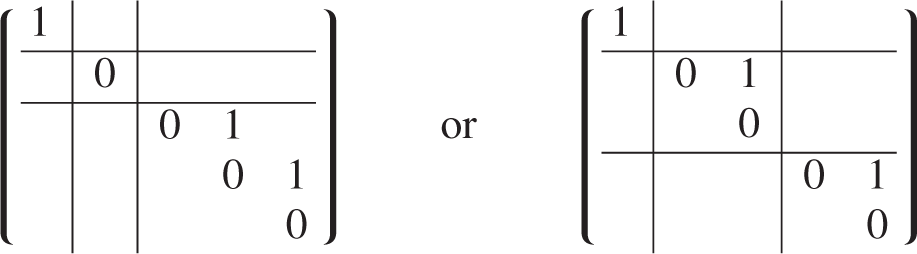
To determine which of these forms is correct, we compute $(A-0I{)}^2=A^2$.

$$A^2=\left[\begin{array}{ccccc}-1& 0& 0& 0& 1\\ -1& 0& 0& 0& 1\\ -1& 0& 0& 0& 1\\ -1& 0& 0& 0& 1\\ -2& 0& 0& 0& 2\end{array}\right]$$

Next we consider the systems

$$A^2\mathbf{x}={\mathbf{x}}_i$$

for $i=2,3$. Since these systems turn out to be inconsistent, the Jordan canonical form of A cannot have any $3\times 3$ simple Jordan blocks and, consequently, it must be of the form

To find X, we must solve

$$A\mathbf{x}={\mathbf{x}}_i$$

for $i=2,3$. The system $A\mathbf{x}={\mathbf{x}}_2$ has infinitely many solutions. We need choose only one of these, say, ${\mathbf{x}}_4=(1,3,0,0,1{)}^T$. Similarly, $A\mathbf{x}={\mathbf{x}}_3$ has infinitely many solutions, one of which is ${\mathbf{x}}_5=(1,0,0,2,1{)}^T$. Let

$$X=\left[\begin{array}{ccccc}{\mathbf{x}}_1& {\mathbf{x}}_2& {\mathbf{x}}_3& {\mathbf{x}}_4& {\mathbf{x}}_5\end{array}\right]=\left[\begin{array}{ccccc}1& 1& 0& 1& 1\\ 1& 1& 0& 3& 0\\ 1& 0& 1& 0& 0\\ 1& 1& 0& 0& 2\\ 2& 1& 0& 1& 1\end{array}\right]$$

The reader may verify that $X^{-1}\mathit{\text{AX}}=J$.

One of the main applications of the Jordan canonical form is in solving systems of linear differential equations that have defective coefficient matrices. Given such a system

we can simplify it by using the Jordan canonical form of A. Indeed, if $A={\mathit{\text{XJX}}}^{-1}$, then

Thus, if we set $\mathbf{Z}={\mathit{\text{X}}}^{-1}\mathbf{Y}$, then $\mathbf{Y}\prime =\text{X}\mathbf{Z}\prime$ and the system simplifies to

Multiplying by $X^{-1}$, we get

Because of the structure of J, this new system is much easier to solve. Indeed, solving (4) will only involve solving a number of smaller systems, each of the form

These equations can be solved one at a time starting with the last. The solution to the last equation is clearly

The solution to any equation of the form

is given by

Thus, we can solve

for $z_{k-1}$ and then solve

for $z_{k-2}$, etc.

The Jordan canonical form not only provides a nice representation of an operator, but it also allows us to solve systems of the form $\mathbf{Y}\prime =A\mathbf{Y}$ even when the coefficient matrix is defective. From a theoretical point of view, its importance cannot be questioned. As far as practical applications go, however, it is generally not very useful.

If $n\ge 5$, it is usually necessary to calculate the eigenvalues of A by some numerical method. The calculated ${\lambda }_i$’s are only approximations to the actual eigenvalues. Thus, we could have calculated values ${\lambda }_1^{\prime }$ and ${\lambda }_2^{\prime }$, which are unequal while actually ${\lambda }_1={\lambda }_2$. So in practice, it may be difficult to determine the correct multiplicity of the eigenvalues. Furthermore, in order to solve $\mathbf{Y}\prime =A\mathbf{Y}$, we need to find the similarity matrix X such that $A={\mathit{\text{XJX}}}^{-1}$. However, when A has multiple eigenvalues, the matrix X may be very sensitive to perturbations and, in practice, one is not guaranteed that the entries of the computed similarity matrix will have any digits of accuracy whatsoever. A recommended alternative is to compute the matrix exponential $e^A$ and use it to solve the system $\mathbf{Y}\prime =A\mathbf{Y}$.