Search in book...
Toggle Font Controls
Create new playlist

Name your new playlist

Playlist description (optional)
Sign In

Email address

Password

Forgot Password?

or

Continue with Facebook

Continue with Google
Sign Up

Full Name

Email address

Confirm Email Address

Password

or

Continue with Facebook

Continue with Google

1.4 Matrix Algebra

The algebraic rules used for real numbers may or may not work when matrices are used. For example, if a and b are real numbers, then

\begin{matrix} a + b = b + a & and & a b = b a \end{matrix}

$\begin{matrix} a + b = b + a & and & a b = b a \end{matrix}$

For real numbers, the operations of addition and multiplication are both commutative. The first of these algebraic rules works when we replace a and b by square matrices A and B, that is,

A + B = B + A

$A + B = B + A$

However, we have already seen that matrix multiplication is not commutative. This fact deserves special emphasis.

In this section, we examine which algebraic rules work for matrices and which do not.

Algebraic Rules

The following theorem provides some useful rules for doing matrix algebra.

Theorem 1.4.1

Each of the following statements is valid for any scalars α and β and for any matrices A, B, and C for which the indicated operations are defined.

$A + B = B + A$ $A + B = B + A$
$(A + B) + C = A + (B + C)$ $(A + B) + C = A + (B + C)$
$(A B) C = A (B C)$ $(A B) C = A (B C)$
$A (B + C) = A B + A C$ $A (B + C) = A B + A C$
$(A + B) C = A C + B C$ $(A + B) C = A C + B C$
$(α β) A = α (β A)$ $(α β) A = α (β A)$
$α (A B) = (α A) B = A (α B)$ $α (A B) = (α A) B = A (α B)$
$(α + β) A = α A + β A$ $(α + β) A = α A + β A$
$α (A + B) = α A + α B$ $α (A + B) = α A + α B$

We will prove two of the rules and leave the rest for the reader to verify.

Proof of Rule 4

Assume that $A = (a_{i j})$ $A = (a_{i j})$ is an $m \times n$ $m \times n$ matrix and $B = (b_{i j})$ $B = (b_{i j})$ and $C = (c_{i j})$ $C = (c_{i j})$ are both $n \times r$ $n \times r$ matrices. Let $D = A (B + C)$ $D = A (B + C)$ and $E = A B + A C$ $E = A B + A C$ . It follows that

d_{i j} = \sum_{k = 1}^{n} a_{i k} (b_{k j} + c_{k j})

$d_{i j} = \sum_{k = 1}^{n} a_{i k} (b_{k j} + c_{k j})$

and

e_{i j} = \sum_{k = 1}^{n} a_{i k} b_{k j} + \sum_{k = 1}^{n} a_{i k} c_{k j}

$e_{i j} = \sum_{k = 1}^{n} a_{i k} b_{k j} + \sum_{k = 1}^{n} a_{i k} c_{k j}$

But

\sum_{k = 1}^{n} a_{i k} (b_{k j} + c_{k j}) = \sum_{k = 1}^{n} a_{i k} b_{k j} + \sum_{k = 1}^{n} a_{i k} c_{k j}

$\sum_{k = 1}^{n} a_{i k} (b_{k j} + c_{k j}) = \sum_{k = 1}^{n} a_{i k} b_{k j} + \sum_{k = 1}^{n} a_{i k} c_{k j}$

so that $d_{i j} = e_{i j}$ $d_{i j} = e_{i j}$ and hence $A (B + C) = A B + A C$ $A (B + C) = A B + A C$ .

∎

Proof of Rule 3

Let A be an $m \times n$ $m \times n$ matrix, B an $n \times r$ $n \times r$ matrix, and C an $r \times s$ $r \times s$ matrix. Let $D = A B$ $D = A B$ and $E = B C$ $E = B C$ . We must show that $D C = A E$ $D C = A E$ . By the definition of matrix multiplication,

d_{i l} = \sum_{k = 1}^{n} a_{i k} b_{k l} and e_{k j} = \sum_{l = 1}^{r} b_{k l} c_{l j}

$d_{i l} = \sum_{k = 1}^{n} a_{i k} b_{k l} and e_{k j} = \sum_{l = 1}^{r} b_{k l} c_{l j}$

The ijth term of DC is

\sum_{l = 1}^{r} d_{i l} c_{l j} = \sum_{l = 1}^{r} (\sum_{k = 1}^{n} a_{i k} b_{k l}) c_{l j}

$\sum_{l = 1}^{r} d_{i l} c_{l j} = \sum_{l = 1}^{r} (\sum_{k = 1}^{n} a_{i k} b_{k l}) c_{l j}$

and the (i, j) entry of AE is

\sum_{k = 1}^{n} a_{i k} e_{k j} = \sum_{k = 1}^{n} a_{i k} (\sum_{l = 1}^{r} b_{k l} c_{l j})

$\sum_{k = 1}^{n} a_{i k} e_{k j} = \sum_{k = 1}^{n} a_{i k} (\sum_{l = 1}^{r} b_{k l} c_{l j})$

Since

\sum_{l = 1}^{r} (\sum_{k = 1}^{n} a_{i k} b_{k l}) c_{l j} = \sum_{l = 1}^{r} (\sum_{k = 1}^{n} a_{i k} b_{k l} c_{l j}) = \sum_{k = 1}^{n} a_{i k} (\sum_{l = 1}^{r} b_{k l} c_{l j})

$\sum_{l = 1}^{r} (\sum_{k = 1}^{n} a_{i k} b_{k l}) c_{l j} = \sum_{l = 1}^{r} (\sum_{k = 1}^{n} a_{i k} b_{k l} c_{l j}) = \sum_{k = 1}^{n} a_{i k} (\sum_{l = 1}^{r} b_{k l} c_{l j})$

it follows that

(A B) C = D C = A E = A (B C)

$(A B) C = D C = A E = A (B C)$

∎

The algebraic rules given in Theorem 1.4.1 seem quite natural, since they are similar to the rules that we use with real numbers. However, there are important differences between the rules for matrix algebra and the algebraic rules for real numbers. Some of these differences are illustrated in Exercises 1 through 5 at the end of this section.

Example 1

\begin{matrix} A = [\begin{matrix} 1 & 2 \\ 3 & 4 \end{matrix}], & B = [\begin{matrix} 2 & 1 \\ - 3 & 2 \end{matrix}], & and & C = [\begin{matrix} 1 & 0 \\ 2 & 1 \end{matrix}] \end{matrix}

$\begin{matrix} A = [\begin{matrix} 1 & 2 \\ 3 & 4 \end{matrix}], & B = [\begin{matrix} 2 & 1 \\ - 3 & 2 \end{matrix}], & and & C = [\begin{matrix} 1 & 0 \\ 2 & 1 \end{matrix}] \end{matrix}$

verify that $A (B C) = (A B) C$ $A (B C) = (A B) C$ and $A (B + C) = A B + A C$ $A (B + C) = A B + A C$ .

SOLUTION

\begin{matrix} A (B C) & = & [\begin{matrix} 1 & 2 \\ 3 & 4 \end{matrix}] [\begin{matrix} 4 & 1 \\ 1 & 2 \end{matrix}] = [\begin{matrix} 6 & 5 \\ 16 & 11 \end{matrix}] \\ (A B) C & = & [\begin{matrix} - 4 & 5 \\ - 6 & 11 \end{matrix}] [\begin{matrix} 1 & 0 \\ 2 & 1 \end{matrix}] = [\begin{matrix} 6 & 5 \\ 16 & 11 \end{matrix}] \end{matrix}

$\begin{matrix} A (B C) & = & [\begin{matrix} 1 & 2 \\ 3 & 4 \end{matrix}] [\begin{matrix} 4 & 1 \\ 1 & 2 \end{matrix}] = [\begin{matrix} 6 & 5 \\ 16 & 11 \end{matrix}] \\ (A B) C & = & [\begin{matrix} - 4 & 5 \\ - 6 & 11 \end{matrix}] [\begin{matrix} 1 & 0 \\ 2 & 1 \end{matrix}] = [\begin{matrix} 6 & 5 \\ 16 & 11 \end{matrix}] \end{matrix}$

Thus,

\begin{matrix} A (B C) & = & [\begin{matrix} 6 & 5 \\ 16 & 11 \end{matrix}] = (A B) C \\ A (B + C) & = & [\begin{matrix} 1 & 2 \\ 3 & 4 \end{matrix}] [\begin{matrix} 3 & 1 \\ - 1 & 3 \end{matrix}] = [\begin{matrix} 1 & 7 \\ 5 & 15 \end{matrix}] \\ A B + A C & = & [\begin{matrix} - 4 & 5 \\ - 6 & 11 \end{matrix}] + [\begin{matrix} 5 & 2 \\ 11 & 4 \end{matrix}] = [\begin{matrix} 1 & 7 \\ 5 & 15 \end{matrix}] \end{matrix}

$\begin{matrix} A (B C) & = & [\begin{matrix} 6 & 5 \\ 16 & 11 \end{matrix}] = (A B) C \\ A (B + C) & = & [\begin{matrix} 1 & 2 \\ 3 & 4 \end{matrix}] [\begin{matrix} 3 & 1 \\ - 1 & 3 \end{matrix}] = [\begin{matrix} 1 & 7 \\ 5 & 15 \end{matrix}] \\ A B + A C & = & [\begin{matrix} - 4 & 5 \\ - 6 & 11 \end{matrix}] + [\begin{matrix} 5 & 2 \\ 11 & 4 \end{matrix}] = [\begin{matrix} 1 & 7 \\ 5 & 15 \end{matrix}] \end{matrix}$

Therefore,

A (B + C) = A B + A C

$A (B + C) = A B + A C$

Notation

Since $(A B) C = A (B C)$ $(A B) C = A (B C)$ , we may simply omit the parentheses and write ABC. The same is true for a product of four or more matrices. In the case where an $n \times n$ $n \times n$ matrix is multiplied by itself a number of times, it is convenient to use exponential notation. Thus, if k is a positive integer, then

A^{k} = \underset{k times}{\underset{︸}{A A \dots A}}

$A^{k} = \underset{k times}{\underset{︸}{A A \dots A}}$

Example 2

A = [\begin{matrix} 1 & 1 \\ 1 & 1 \end{matrix}]

$A = [\begin{matrix} 1 & 1 \\ 1 & 1 \end{matrix}]$

then

\begin{matrix} A^{2} = [\begin{matrix} 1 & 1 \\ 1 & 1 \end{matrix}] [\begin{matrix} 1 & 1 \\ 1 & 1 \end{matrix}] = [\begin{matrix} 2 & 2 \\ 2 & 2 \end{matrix}] \\ A^{3} = A A A = A A^{2} = [\begin{matrix} 1 & 1 \\ 1 & 1 \end{matrix}] [\begin{matrix} 2 & 2 \\ 2 & 2 \end{matrix}] = [\begin{matrix} 4 & 4 \\ 4 & 4 \end{matrix}] \end{matrix}

$\begin{matrix} A^{2} = [\begin{matrix} 1 & 1 \\ 1 & 1 \end{matrix}] [\begin{matrix} 1 & 1 \\ 1 & 1 \end{matrix}] = [\begin{matrix} 2 & 2 \\ 2 & 2 \end{matrix}] \\ A^{3} = A A A = A A^{2} = [\begin{matrix} 1 & 1 \\ 1 & 1 \end{matrix}] [\begin{matrix} 2 & 2 \\ 2 & 2 \end{matrix}] = [\begin{matrix} 4 & 4 \\ 4 & 4 \end{matrix}] \end{matrix}$

and, in general,

A^{n} = [\begin{matrix} 2^{n - 1} & 2^{n - 1} \\ 2^{n - 1} & 2^{n - 1} \end{matrix}]

$A^{n} = [\begin{matrix} 2^{n - 1} & 2^{n - 1} \\ 2^{n - 1} & 2^{n - 1} \end{matrix}]$

Application 1

A Simple Model for Marital Status Computations

In a certain town, 30 percent of the married women get divorced each year and 20 percent of the single women get married each year. There are 8000 married women and 2000 single women. Assuming that the total population of women remains constant, how many married women and how many single women will there be after one year? After two years?

Solution

Form a matrix A as follows: The entries in the first row of A will be the percentages of married and single women, respectively, who are married after one year. The entries in the second row will be the percentages of women who are single after one year. Thus,

A = [\begin{matrix} 0.70 & 0.20 \\ 0.30 & 0.80 \end{matrix}]

$A = [\begin{matrix} 0.70 & 0.20 \\ 0.30 & 0.80 \end{matrix}]$

If we let $x = [\begin{matrix} 8000 \\ 2000 \end{matrix}]$ $x = [\begin{matrix} 8000 \\ 2000 \end{matrix}]$ , the number of married and single women after one year can be computed by multiplying A times x.

A x = [\begin{matrix} 0.70 & 0.20 \\ 0.30 & 0.80 \end{matrix}] [\begin{matrix} 8000 \\ 2000 \end{matrix}] = [\begin{matrix} 6000 \\ 4000 \end{matrix}]

$A x = [\begin{matrix} 0.70 & 0.20 \\ 0.30 & 0.80 \end{matrix}] [\begin{matrix} 8000 \\ 2000 \end{matrix}] = [\begin{matrix} 6000 \\ 4000 \end{matrix}]$

After one year, there will be 6000 married women and 4000 single women. To find the number of married and single women after two years, compute

A^{2} x = A (A x) = [\begin{matrix} 0.70 & 0.20 \\ 0.30 & 0.80 \end{matrix}] [\begin{matrix} 6000 \\ 4000 \end{matrix}] = [\begin{matrix} 5000 \\ 5000 \end{matrix}]

$A^{2} x = A (A x) = [\begin{matrix} 0.70 & 0.20 \\ 0.30 & 0.80 \end{matrix}] [\begin{matrix} 6000 \\ 4000 \end{matrix}] = [\begin{matrix} 5000 \\ 5000 \end{matrix}]$

After two years, half of the women will be married and half will be single. In general, the number of married and single women after n years can be determined by computing $A^{n} x$ $A^{n} x$ .

Application 2

Ecology: Demographics of the Loggerhead Sea Turtle

The management and preservation of many wildlife species depend on our ability to model population dynamics. A standard modeling technique is to divide the life cycle of a species into a number of stages. The models assume that the population sizes for each stage depend only on the female population and that the probability of survival of an individual female from one year to the next depends only on the stage of the life cycle and not on the actual age of an individual. For example, let us consider a four-stage model for analyzing the population dynamics of the loggerhead sea turtle (see Figure 1.4.1).

Figure 1.4.1.

Loggerhead Sea Turtle

Figure 1.4.1. Full Alternative Text

At each stage, we estimate the probability of survival over a one-year period. We also estimate the ability to reproduce in terms of the expected number of eggs laid in a given year. The results are summarized in Table 1.4.1. The approximate ages for each stage are listed in parentheses next to the stage description.

Table 1.4.1 Four-Stage Model for Loggerhead Sea Turtle Demographics

Stage Number	Description (age in years)	Annual Survivorship	Eggs Laid per Year
1	Eggs, hatchlings (<1)	0.67	0
2	Juveniles and subadults (1–21)	0.74	0
3	Novice breeders (22)	0.81	127
4	Mature breeders (23–54)	0.81	79

If $d_{i}$ $d_{i}$ represents the duration of the ith stage and $s_{i}$ $s_{i}$ is the annual survivorship rate for that stage, then it can be shown that the proportion remaining in stage i the following year will be

p_{i} = (\frac{1 - s_{i}^{d_{i} - 1}}{1 - s_{i}^{d_{i}}}) s_{i}

$p_{i} = (\frac{1 - s_{i}^{d_{i} - 1}}{1 - s_{i}^{d_{i}}}) s_{i}$ (1)

and the proportion of the population that will survive and move into stage $i + 1$ $i + 1$ the following year will be

q_{i} = \frac{s_{i}^{d_{i}} (1 - s_{i})}{1 - s_{i}^{d_{i}}}

$q_{i} = \frac{s_{i}^{d_{i}} (1 - s_{i})}{1 - s_{i}^{d_{i}}}$ (2)

If we let $e_{i}$ $e_{i}$ denote the average number of eggs laid by a member of stage $i (i = 2, 3, 4)$ $i (i = 2, 3, 4)$ in one year and form the matrix

L = [\begin{array}{l} p_{1} & e_{2} & e_{3} & e_{4} \\ q_{1} & p_{2} & 0 & 0 \\ 0 & q_{2} & p_{3} & 0 \\ 0 & 0 & q_{3} & p_{4} \end{array}]

$L = [\begin{array}{l} p_{1} & e_{2} & e_{3} & e_{4} \\ q_{1} & p_{2} & 0 & 0 \\ 0 & q_{2} & p_{3} & 0 \\ 0 & 0 & q_{3} & p_{4} \end{array}]$ (3)

then L can be used to predict the turtle populations at each stage in future years. A matrix of the form (3) is called a Leslie matrix, and the corresponding population model is sometimes referred to as a Leslie population model. Using the figures from Table 1.4.1, the Leslie matrix for our model is

L = [\begin{matrix} 0 & 0 & 127 & 79 \\ 0.67 & 0.7394 & 0 & 0 \\ 0 & 0.006 & 0 & 0 \\ 0 & 0 & 0.81 & 0.8097 \end{matrix}]

$L = [\begin{matrix} 0 & 0 & 127 & 79 \\ 0.67 & 0.7394 & 0 & 0 \\ 0 & 0.006 & 0 & 0 \\ 0 & 0 & 0.81 & 0.8097 \end{matrix}]$

Suppose that the initial populations at each stage were 200,000, 300,000, 500, and 1500, respectively. If we represent these initial populations by a vector $x_{0}$ $x_{0}$ , the populations at each stage after one year are determined by computing

x = L x_{0} = [\begin{matrix} 0 & 0 & 127 & 79 \\ 0.67 & 0.7394 & 0 & 0 \\ 0 & 0.0006 & 0 & 0 \\ 0 & 0 & 0.81 & 0.8097 \end{matrix}] [\begin{array}{r} 200, 000 \\ 300, 000 \\ 500 \\ 1500 \end{array}] = [\begin{array}{r} 182, 000 \\ 355, 820 \\ 180 \\ 1620 \end{array}]

$x = L x_{0} = [\begin{matrix} 0 & 0 & 127 & 79 \\ 0.67 & 0.7394 & 0 & 0 \\ 0 & 0.0006 & 0 & 0 \\ 0 & 0 & 0.81 & 0.8097 \end{matrix}] [\begin{array}{r} 200, 000 \\ 300, 000 \\ 500 \\ 1500 \end{array}] = [\begin{array}{r} 182, 000 \\ 355, 820 \\ 180 \\ 1620 \end{array}]$

(The computations have been rounded to the nearest integer.) To determine the population vector after two years, we multiply again by the matrix L.

x_{2} = L x_{1} = L^{2} x_{0}

$x_{2} = L x_{1} = L^{2} x_{0}$

In general, the population after k years is determined by computing $x_{k} = L^{k} x_{0}$ $x_{k} = L^{k} x_{0}$ . To see longer-range trends, we compute $x_{10}$ $x_{10}$ , $x_{25}$ $x_{25}$ , $x_{50}$ $x_{50}$ , and $x_{100}$ $x_{100}$ . The results are summarized in Table 1.4.2. The model predicts that the total number of breeding-age turtles will decrease by approximately 95 percent over a 100-year period.

Table 1.4.2 Loggerhead Sea Turtle Population Projections

Stage Number	Initial Population	10 Years	25 Years	50 Years	100 Years
1	200,000	115,403	75,768	37,623	9276
2	300,000	331,274	217,858	108,178	26,673
3	500	215	142	70	17
4	1500	1074	705	350	86

A seven-stage model describing the population dynamics is presented in reference [1] that follows. We will use the seven-stage model in the computer exercises at the end of this chapter. Reference [2] is the original paper by Leslie.

References

1. Crouse, Deborah T., Larry B. Crowder, and Hal Caswell, “A Stage-Based Population Model for Loggerhead Sea Turtles and Implications for Conservation,” Ecology, 68(5), 1987.
2. Leslie, P. H., “On the Use of Matrices in Certain Population Mathematics,” Biometrika, 33, 1945.

The Identity Matrix

Just as the number 1 acts as an identity for the multiplication of real numbers, there is a special matrix I that acts as an identity for matrix multiplication; that is,

I A = A I = A

$I A = A I = A$ (4)

for any $n \times n$ $n \times n$ matrix A. It is easy to verify that, if we define I to be an $n \times n$ $n \times n$ matrix with 1’s on the main diagonal and 0’s elsewhere, then I satisfies equation (4) for any $n \times n$ $n \times n$ matrix A. More formally, we have the following definition.

As an example, let us verify equation (4) in the case $n = 3$ $n = 3$ :

[\begin{matrix} 1 & 0 & 0 \\ 0 & 1 & 0 \\ 0 & 0 & 1 \end{matrix}] [\begin{matrix} 3 & 4 & 1 \\ 2 & 6 & 3 \\ 0 & 1 & 8 \end{matrix}] = [\begin{matrix} 3 & 4 & 1 \\ 2 & 6 & 3 \\ 0 & 1 & 8 \end{matrix}]

$[\begin{matrix} 1 & 0 & 0 \\ 0 & 1 & 0 \\ 0 & 0 & 1 \end{matrix}] [\begin{matrix} 3 & 4 & 1 \\ 2 & 6 & 3 \\ 0 & 1 & 8 \end{matrix}] = [\begin{matrix} 3 & 4 & 1 \\ 2 & 6 & 3 \\ 0 & 1 & 8 \end{matrix}]$

and

[\begin{matrix} 3 & 4 & 1 \\ 2 & 6 & 3 \\ 0 & 1 & 8 \end{matrix}] [\begin{matrix} 1 & 0 & 0 \\ 0 & 1 & 0 \\ 0 & 0 & 1 \end{matrix}] = [\begin{matrix} 3 & 4 & 1 \\ 2 & 6 & 3 \\ 0 & 1 & 8 \end{matrix}]

$[\begin{matrix} 3 & 4 & 1 \\ 2 & 6 & 3 \\ 0 & 1 & 8 \end{matrix}] [\begin{matrix} 1 & 0 & 0 \\ 0 & 1 & 0 \\ 0 & 0 & 1 \end{matrix}] = [\begin{matrix} 3 & 4 & 1 \\ 2 & 6 & 3 \\ 0 & 1 & 8 \end{matrix}]$

In general, if B is any $m \times n$ $m \times n$ matrix and C is any $n \times r$ $n \times r$ matrix, then

\begin{matrix} B I = B & and & I C = C \end{matrix}

$\begin{matrix} B I = B & and & I C = C \end{matrix}$

The column vectors of the $n \times n$ $n \times n$ identity matrix I are the standard vectors used to define a coordinate system in Euclidean n-space. The standard notation for the jth column vector of I is $e_{j}$ $e_{j}$ , rather than the usual $i_{j}$ $i_{j}$ . Thus, the $n \times n$ $n \times n$ identity matrix can be written

I = (e_{1}, e_{2}, \dots, e_{n})

$I = (e_{1}, e_{2}, \dots, e_{n})$

Matrix Inversion

A real number a is said to have a multiplicative inverse if there exists a number b such that $ab = 1$ $ab = 1$ . Any nonzero number a has a multiplicative inverse $b = \frac{1}{a}$ $b = \frac{1}{a}$ . We generalize the concept of multiplicative inverses to matrices with the following definition.

If B and C are both multiplicative inverses of A, then

B = B I = B (A C) = (B A) C = I C = C

$B = B I = B (A C) = (B A) C = I C = C$

Thus, a matrix can have at most one multiplicative inverse. We will refer to the multiplicative inverse of a nonsingular matrix A as simply the inverse of A and denote it by $A^{- 1}$ $A^{- 1}$ .

Example 3

The matrices

\begin{matrix} [\begin{matrix} 2 & 4 \\ 3 & 1 \end{matrix}] & and & [\begin{matrix} - \frac{1}{10} & \frac{2}{5} \\ \frac{3}{10} & - \frac{1}{5} \end{matrix}] \end{matrix}

$\begin{matrix} [\begin{matrix} 2 & 4 \\ 3 & 1 \end{matrix}] & and & [\begin{matrix} - \frac{1}{10} & \frac{2}{5} \\ \frac{3}{10} & - \frac{1}{5} \end{matrix}] \end{matrix}$

are inverses of each other, since

\begin{matrix} [\begin{matrix} 2 & 4 \\ 3 & 1 \end{matrix}] \end{matrix} \begin{matrix} [\begin{matrix} - \frac{1}{10} & \frac{2}{5} \\ \frac{3}{10} & - \frac{1}{5} \end{matrix}] \end{matrix} = [\begin{matrix} 1 & 0 \\ 0 & 1 \end{matrix}]

$\begin{matrix} [\begin{matrix} 2 & 4 \\ 3 & 1 \end{matrix}] \end{matrix} \begin{matrix} [\begin{matrix} - \frac{1}{10} & \frac{2}{5} \\ \frac{3}{10} & - \frac{1}{5} \end{matrix}] \end{matrix} = [\begin{matrix} 1 & 0 \\ 0 & 1 \end{matrix}]$

and

\begin{matrix} [\begin{matrix} - \frac{1}{10} & \frac{2}{5} \\ \frac{3}{10} & - \frac{1}{5} \end{matrix}] \end{matrix} \begin{matrix} [\begin{matrix} 2 & 4 \\ 3 & 1 \end{matrix}] \end{matrix} = [\begin{matrix} 1 & 0 \\ 0 & 1 \end{matrix}]

$\begin{matrix} [\begin{matrix} - \frac{1}{10} & \frac{2}{5} \\ \frac{3}{10} & - \frac{1}{5} \end{matrix}] \end{matrix} \begin{matrix} [\begin{matrix} 2 & 4 \\ 3 & 1 \end{matrix}] \end{matrix} = [\begin{matrix} 1 & 0 \\ 0 & 1 \end{matrix}]$

Example 4

The $3 \times 3$ $3 \times 3$ matrices

\begin{matrix} [\begin{matrix} 1 & 2 & 3 \\ 0 & 1 & 4 \\ 0 & 0 & 1 \end{matrix}] & and & [\begin{matrix} 1 & - 2 & 5 \\ 0 & 1 & - 4 \\ 0 & 0 & 1 \end{matrix}] \end{matrix}

$\begin{matrix} [\begin{matrix} 1 & 2 & 3 \\ 0 & 1 & 4 \\ 0 & 0 & 1 \end{matrix}] & and & [\begin{matrix} 1 & - 2 & 5 \\ 0 & 1 & - 4 \\ 0 & 0 & 1 \end{matrix}] \end{matrix}$

are inverses, since

\begin{matrix} [\begin{matrix} 1 & 2 & 3 \\ 0 & 1 & 4 \\ 0 & 0 & 1 \end{matrix}] \end{matrix} \begin{matrix} [\begin{matrix} 1 & - 2 & 5 \\ 0 & 1 & - 4 \\ 0 & 0 & 1 \end{matrix}] \end{matrix} = \begin{matrix} [\begin{matrix} 1 & 0 & 0 \\ 0 & 1 & 0 \\ 0 & 0 & 1 \end{matrix}] \end{matrix}

$\begin{matrix} [\begin{matrix} 1 & 2 & 3 \\ 0 & 1 & 4 \\ 0 & 0 & 1 \end{matrix}] \end{matrix} \begin{matrix} [\begin{matrix} 1 & - 2 & 5 \\ 0 & 1 & - 4 \\ 0 & 0 & 1 \end{matrix}] \end{matrix} = \begin{matrix} [\begin{matrix} 1 & 0 & 0 \\ 0 & 1 & 0 \\ 0 & 0 & 1 \end{matrix}] \end{matrix}$

and

\begin{matrix} [\begin{matrix} 1 & - 2 & 5 \\ 0 & 1 & - 4 \\ 0 & 0 & 1 \end{matrix}] \end{matrix} \begin{matrix} [\begin{matrix} 1 & 2 & 3 \\ 0 & 1 & 4 \\ 0 & 0 & 1 \end{matrix}] \end{matrix} = \begin{matrix} [\begin{matrix} 1 & 0 & 0 \\ 0 & 1 & 0 \\ 0 & 0 & 1 \end{matrix}] \end{matrix}

$\begin{matrix} [\begin{matrix} 1 & - 2 & 5 \\ 0 & 1 & - 4 \\ 0 & 0 & 1 \end{matrix}] \end{matrix} \begin{matrix} [\begin{matrix} 1 & 2 & 3 \\ 0 & 1 & 4 \\ 0 & 0 & 1 \end{matrix}] \end{matrix} = \begin{matrix} [\begin{matrix} 1 & 0 & 0 \\ 0 & 1 & 0 \\ 0 & 0 & 1 \end{matrix}] \end{matrix}$

Example 5

The matrix

A = [\begin{matrix} 1 & 0 \\ 0 & 0 \end{matrix}]

$A = [\begin{matrix} 1 & 0 \\ 0 & 0 \end{matrix}]$

has no inverse. Indeed, if B is any $2 \times 2$ $2 \times 2$ matrix, then

B A = [\begin{matrix} b_{11} & b_{12} \\ b_{21} & b_{22} \end{matrix}] [\begin{matrix} 1 & 0 \\ 0 & 0 \end{matrix}] = [\begin{matrix} b_{11} & 0 \\ b_{21} & 0 \end{matrix}]

$B A = [\begin{matrix} b_{11} & b_{12} \\ b_{21} & b_{22} \end{matrix}] [\begin{matrix} 1 & 0 \\ 0 & 0 \end{matrix}] = [\begin{matrix} b_{11} & 0 \\ b_{21} & 0 \end{matrix}]$

Thus, BA cannot equal I.

Note

Only square matrices have multiplicative inverses. One should not use the terms singular and nonsingular when referring to nonsquare matrices.

Often we will be working with products of nonsingular matrices. It turns out that any product of nonsingular matrices is nonsingular. The following theorem characterizes how the inverse of the product of a pair of nonsingular matrices A and B is related to the inverses of A and B:

Theorem 1.4.2

If A and B are nonsingular $n \times n$ $n \times n$ matrices, then AB is also nonsingular and $(A B)^{- 1} = B^{- 1} A^{- 1}$ $(A B)^{- 1} = B^{- 1} A^{- 1}$ .

Proof

\begin{matrix} (B^{- 1} A^{- 1}) A B = B^{- 1} (A^{- 1} A) B = B^{- 1} B = I \\ (A B) (B^{- 1} A^{- 1}) = A (B B^{- 1}) A^{- 1} = A A^{- 1} = I \end{matrix}

$\begin{matrix} (B^{- 1} A^{- 1}) A B = B^{- 1} (A^{- 1} A) B = B^{- 1} B = I \\ (A B) (B^{- 1} A^{- 1}) = A (B B^{- 1}) A^{- 1} = A A^{- 1} = I \end{matrix}$

∎

It follows by induction that, if $A_{1}, \dots, A_{k}$ $A_{1}, \dots, A_{k}$ are all nonsingular $n \times n$ $n \times n$ matrices, then the product $A_{1} A_{2} \dots A_{k}$ $A_{1} A_{2} \dots A_{k}$ is nonsingular and

{(A_{1} A_{2} \dots A_{k})}^{- 1} = A_{k}^{- 1} \dots A_{2}^{- 1} A_{1}^{- 1}

${(A_{1} A_{2} \dots A_{k})}^{- 1} = A_{k}^{- 1} \dots A_{2}^{- 1} A_{1}^{- 1}$

In the next section, we will learn how to determine whether a matrix has a multiplicative inverse. We will also learn a method for computing the inverse of a nonsingular matrix.

Algebraic Rules for Transposes

There are four basic algebraic rules involving transposes.

Algebraic Rules for Transposes

$(A^{T})^{T} = A$ $(A^{T})^{T} = A$
$(α A)^{T} = α A^{T}$ $(α A)^{T} = α A^{T}$
$(A + B)^{T} = A^{T} + B^{T}$ $(A + B)^{T} = A^{T} + B^{T}$
$(A B)^{T} = B^{T} A^{T}$ $(A B)^{T} = B^{T} A^{T}$

The first three rules are straightforward. We leave it to the reader to verify that they are valid. To prove the fourth rule, we need only show that the (i, j) entries of $(A B)^{T}$ $(A B)^{T}$ and $B^{T} A^{T}$ $B^{T} A^{T}$ are equal. If A is an $m \times n$ $m \times n$ matrix, then, for the multiplications to be possible, B must have n rows. The (i, j) entry of $(A B)^{T}$ $(A B)^{T}$ is the (j, i) entry of AB. It is computed by multiplying the jth row vector of A times the ith column vector of B:

{\vec{a}}_{j} b_{i} = (a_{j 1}, a_{j 2}, \dots, a_{j n}) [\begin{matrix} b_{1 i} \\ b_{2 i} \\ ⋮ \\ b_{n i} \end{matrix}] = a_{j 1} b_{1 i} + a_{j 2} b_{2 i} + \dots + a_{j n} b_{n i}

${\vec{a}}_{j} b_{i} = (a_{j 1}, a_{j 2}, \dots, a_{j n}) [\begin{matrix} b_{1 i} \\ b_{2 i} \\ ⋮ \\ b_{n i} \end{matrix}] = a_{j 1} b_{1 i} + a_{j 2} b_{2 i} + \dots + a_{j n} b_{n i}$ (5)

The (i, j) entry of $B^{T} A^{T}$ $B^{T} A^{T}$ is computed by multiplying the ith row of $B^{T}$ $B^{T}$ times the jth column of $A^{T}$ $A^{T}$ . Since the ith row of $B^{T}$ $B^{T}$ is the transpose of the ith column of B and the jth column of $A^{T}$ $A^{T}$ is the transpose of the jth row of A, it follows that the (i, j) entry of $B^{T} A^{T}$ $B^{T} A^{T}$ is given by

b_{i}^{T} {\vec{a}}_{j}^{T} = (b_{1 i}, b_{2 i}, \dots, b_{n i}) [\begin{matrix} a_{j 1} \\ a_{j 2} \\ ⋮ \\ a_{j n} \end{matrix}] = b_{1 i} a_{j 1} + b_{2 i} a_{j 2} + \dots + b_{n i} a_{j n}

$b_{i}^{T} {\vec{a}}_{j}^{T} = (b_{1 i}, b_{2 i}, \dots, b_{n i}) [\begin{matrix} a_{j 1} \\ a_{j 2} \\ ⋮ \\ a_{j n} \end{matrix}] = b_{1 i} a_{j 1} + b_{2 i} a_{j 2} + \dots + b_{n i} a_{j n}$ (6)

It follows from (5) and (6) that the (i, j) entries of $(A B)^{T}$ $(A B)^{T}$ and $B^{T} A^{T}$ $B^{T} A^{T}$ are equal.

The next example illustrates the idea behind the last proof.

Example 6

Let

\begin{matrix} A = [\begin{matrix} 1 & 2 & 1 \\ 3 & 3 & 5 \\ 2 & 4 & 1 \end{matrix}], & B = [\begin{matrix} 1 & 0 & 2 \\ 2 & 1 & 1 \\ 5 & 4 & 1 \end{matrix}] \end{matrix}

$\begin{matrix} A = [\begin{matrix} 1 & 2 & 1 \\ 3 & 3 & 5 \\ 2 & 4 & 1 \end{matrix}], & B = [\begin{matrix} 1 & 0 & 2 \\ 2 & 1 & 1 \\ 5 & 4 & 1 \end{matrix}] \end{matrix}$

Note that, on the one hand, the (3, 2) entry of AB is computed taking the scalar product of the third row of A and the second column of B.

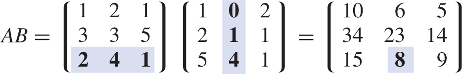
Matrix multiplication of two 3 by 3 augmented matrices, A and B.

1.7-28 Full Alternative Text

When the product is transposed, the (3, 2) entry of AB becomes the (2, 3) entry of $(A B)^{T}$ $(A B)^{T}$ .

(A B)^{T} = [\begin{matrix} 10 & 34 & 15 \\ 6 & 23 & 8 \\ 5 & 14 & 9 \end{matrix}]

$(A B)^{T} = [\begin{matrix} 10 & 34 & 15 \\ 6 & 23 & 8 \\ 5 & 14 & 9 \end{matrix}]$

On the other hand, the (2, 3) entry of $B^{T} A^{T}$ $B^{T} A^{T}$ is computed taking the scalar product of the second row of $B^{T}$ $B^{T}$ and the third column of $A^{T}$ $A^{T}$ .

Matrix multiplication of two 3 by 3 augmented matrices B to the power of T and A to the power of T.

1.7-29 Full Alternative Text

In both cases, the arithmetic for computing the (2, 3) entry is the same.

Symmetric Matrices and Networks

Recall that a matrix A is symmetric if $A^{T} = A$ $A^{T} = A$ . One type of application that leads to symmetric matrices is problems involving networks. These problems are often solved using the techniques of an area of mathematics called graph theory.

Application 3

Networks and Graphs

Graph theory is an important area of applied mathematics. It is used to model problems in virtually all the applied sciences. Graph theory is particularly useful in applications involving communications networks.

A graph is defined to be a set of points called vertices, together with a set of unordered pairs of vertices, which are referred to as edges. Figure 1.4.2 gives a geometrical representation of a graph. We can think of the vertices $V_{1}$ $V_{1}$ , $V_{2}$ $V_{2}$ , $V_{3}$ $V_{3}$ , $V_{4}$ $V_{4}$ , and $V_{5}$ $V_{5}$ as corresponding to the nodes in a communications network.

Figure 1.4.2.

Figure 1.4.2. Full Alternative Text

The line segments joining the vertices correspond to the edges:

{V_{1}, V_{2}}, {V_{2}, V_{5}}, {V_{3}, V_{4}}, {V_{3}, V_{5}}, {V_{4}, V_{5}}

${V_{1}, V_{2}}, {V_{2}, V_{5}}, {V_{3}, V_{4}}, {V_{3}, V_{5}}, {V_{4}, V_{5}}$

Each edge represents a direct communications link between two nodes of the network.

An actual communications network could involve a large number of vertices and edges. Indeed, if there are millions of vertices, a graphical picture of the network would be quite confusing. An alternative is to use a matrix representation for the network. If the graph contains a total of n vertices, we can define an $n \times n$ $n \times n$ matrix A by

a_{i j} = {\begin{matrix} 1 & if {V_{i}, V_{j}} is an edge of the graph \\ 0 & if there is no edge joining V_{i} and V_{j} \end{matrix}

$a_{i j} = {\begin{matrix} 1 & if {V_{i}, V_{j}} is an edge of the graph \\ 0 & if there is no edge joining V_{i} and V_{j} \end{matrix}$

The matrix A is called the adjacency matrix of the graph. The adjacency matrix for the graph in Figure 1.4.2 is given by

A = [\begin{matrix} 0 & 1 & 0 & 0 & 0 \\ 1 & 0 & 0 & 0 & 1 \\ 0 & 0 & 0 & 1 & 1 \\ 0 & 0 & 1 & 0 & 1 \\ 0 & 1 & 1 & 1 & 0 \end{matrix}]

$A = [\begin{matrix} 0 & 1 & 0 & 0 & 0 \\ 1 & 0 & 0 & 0 & 1 \\ 0 & 0 & 0 & 1 & 1 \\ 0 & 0 & 1 & 0 & 1 \\ 0 & 1 & 1 & 1 & 0 \end{matrix}]$

Note that the matrix A is symmetric. Indeed, any adjacency matrix must be symmetric, for if ${V_{i}, V_{j}}$ ${V_{i}, V_{j}}$ is an edge of the graph, then $a_{i j} = a_{j i} = 1$ $a_{i j} = a_{j i} = 1$ and $a_{i j} = a_{j i} = 0$ $a_{i j} = a_{j i} = 0$ if there is no edge joining $V_{i}$ $V_{i}$ and $V_{j}$ $V_{j}$ . In either case, $a_{i j} = a_{j i}$ $a_{i j} = a_{j i}$ .

We can think of a walk in a graph as a sequence of edges linking one vertex to another. For example, in Figure 1.4.2 the edges ${V_{1}, V_{2}}, {V_{2}, V_{5}}$ ${V_{1}, V_{2}}, {V_{2}, V_{5}}$ represent a walk from vertex $V_{1}$ $V_{1}$ to vertex $V_{5}$ $V_{5}$ . The length of the walk is said to be 2 since it consists of two edges. A simple way to describe the walk is to indicate the movement between vertices by arrows. Thus, $V_{1} \to V_{2} \to V_{5}$ $V_{1} \to V_{2} \to V_{5}$ denotes a walk of length 2 from $V_{1}$ $V_{1}$ to $V_{5}$ $V_{5}$ . Similarly, $V_{4} \to V_{5} \to V_{2} \to V_{1}$ $V_{4} \to V_{5} \to V_{2} \to V_{1}$ represents a walk of length 3 from $V_{4}$ $V_{4}$ to $V_{1}$ $V_{1}$ . It is possible to traverse the same edges more than once in a walk. For example, $V_{5} \to V_{3} \to V_{5} \to V_{3}$ $V_{5} \to V_{3} \to V_{5} \to V_{3}$ is a walk of length 3 from $V_{5}$ $V_{5}$ to $V_{3}$ $V_{3}$ . In general, by taking powers of the adjacency matrix, we can determine the number of walks of any specified length between two vertices.

Theorem 1.4.3

If A is an $n \times n$ $n \times n$ adjacency matrix of a graph and $a_{i j}^{(k)}$ $a_{i j}^{(k)}$ represents the (i, j) entry of $A^{k}$ $A^{k}$ , then $a_{i j}^{(k)}$ $a_{i j}^{(k)}$ is equal to the number of walks of length k from $V_{i}$ $V_{i}$ to $V_{j}$ $V_{j}$ .

Proof

The proof is by mathematical induction. In the case $k = 1$ $k = 1$ , it follows from the definition of the adjacency matrix that $a_{i j}$ $a_{i j}$ represents the number of walks of length 1 from $V_{i}$ $V_{i}$ to $V_{j}$ $V_{j}$ . Assume for some m that each entry of $A^{m}$ $A^{m}$ is equal to the number of walks of length m between the corresponding vertices. Thus, $a_{i l}^{(m)}$ $a_{i l}^{(m)}$ is the number of walks of length m from $V_{i}$ $V_{i}$ to $V_{l}$ $V_{l}$ . Now on the one hand, if there is an edge ${V_{l}, V_{j}}$ ${V_{l}, V_{j}}$ , then $a_{i l}^{(m)} a_{l j} = a_{i l}^{(m)}$ $a_{i l}^{(m)} a_{l j} = a_{i l}^{(m)}$ is the number of walks of length $m + 1$ $m + 1$ from $V_{i}$ $V_{i}$ to $V_{j}$ $V_{j}$ of the form

V_{i} \to \dots \to V_{l} \to V_{j}

$V_{i} \to \dots \to V_{l} \to V_{j}$

On the other hand, if ${V_{l}, V_{j}}$ ${V_{l}, V_{j}}$ is not an edge, then there are no walks of length $m + 1$ $m + 1$ of this form from $V_{i}$ $V_{i}$ to $V_{j}$ $V_{j}$ and

a_{i l}^{(m)} a_{l j} = a_{i l}^{(m)} \cdot 0 = 0

$a_{i l}^{(m)} a_{l j} = a_{i l}^{(m)} \cdot 0 = 0$

It follows that the total number of walks of length $m + 1$ $m + 1$ from $V_{i}$ $V_{i}$ to $V_{j}$ $V_{j}$ is given by

a_{i 1}^{(m)} a_{1 j} + a_{i 2}^{(m)} a_{2 j} + \dots + a_{i n}^{(m)} a_{n j}

$a_{i 1}^{(m)} a_{1 j} + a_{i 2}^{(m)} a_{2 j} + \dots + a_{i n}^{(m)} a_{n j}$

But this is just the (i, j) entry of $A^{m + 1}$ $A^{m + 1}$ .

∎

Example 7

To determine the number of walks of length 3 between any two vertices of the graph in Figure 1.4.2, we need only compute

A^{3} = [\begin{matrix} 0 & 2 & 1 & 1 & 0 \\ 2 & 0 & 1 & 1 & 4 \\ 1 & 1 & 2 & 3 & 4 \\ 1 & 1 & 3 & 2 & 4 \\ 0 & 4 & 4 & 4 & 2 \end{matrix}]

$A^{3} = [\begin{matrix} 0 & 2 & 1 & 1 & 0 \\ 2 & 0 & 1 & 1 & 4 \\ 1 & 1 & 2 & 3 & 4 \\ 1 & 1 & 3 & 2 & 4 \\ 0 & 4 & 4 & 4 & 2 \end{matrix}]$

Thus, the number of walks of length 3 from $V_{3}$ $V_{3}$ to $V_{5}$ $V_{5}$ is $a_{35}^{(3)} = 4$ $a_{35}^{(3)} = 4$ . Note that the matrix $A^{3}$ $A^{3}$ is symmetric. This reflects the fact that there are the same number of walks of length 3 from $V_{i}$ $V_{i}$ to $V_{j}$ $V_{j}$ as there are from $V_{j}$ $V_{j}$ to $V_{i}$ $V_{i}$ .

..................Content has been hidden....................

You can't read the all page of ebook, please click here login for view all page.

Table of Contents for 1.4 Matrix Algebra

Create new playlist

Sign In

Sign Up

Table of Contents for
1.4 Matrix Algebra