Search in book...
Toggle Font Controls
Create new playlist

Name your new playlist

Playlist description (optional)
Sign In

Email address

Password

Forgot Password?

or

Continue with Facebook

Continue with Google
Sign Up

Full Name

Email address

Confirm Email Address

Password

or

Continue with Facebook

Continue with Google

5.5 Orthonormal Sets

In R2 $ℝ^{2}$ , it is generally more convenient to use the standard basis {e1,e2} ${e_{1}, e_{2}}$ than to use some other basis, such as {(2,1)T,(3,5)T} ${{(2, 1)}^{T}, {(3, 5)}^{T}}$ . For example, it would be easier to find the coordinates of (x1,x2)T ${(x_{1}, x_{2})}^{T}$ with respect to the standard basis. The elements of the standard basis are orthogonal unit vectors. In working with an inner product space V, it is generally desirable to have a basis of mutually orthogonal unit vectors. Such a basis is convenient not only in finding coordinates of vectors, but also in solving least squares problems.

Example 1

The set {(1,1,1)T,(2,1,−3)T,(4,−5,1)T} ${{(1, 1, 1)}^{T}, {(2, 1, - 3)}^{T}, {(4, - 5, 1)}^{T}}$ is an orthogonal set in R3 $ℝ^{3}$ , since

(1, 1, 1) (2, 1, - 3) T (1, 1, 1) (4, - 5, 1) T (2, 1, - 3) (4, - 5, 1) T = 0 = 0 = 0

$\begin{matrix} (1, 1, 1) {(2, 1, - 3)}^{T} & = 0 \\ (1, 1, 1) {(4, - 5, 1)}^{T} & = 0 \\ (2, 1, - 3) {(4, - 5, 1)}^{T} & = 0 \end{matrix}$

Theorem 5.5.1

If {v1,v2,…,vn} ${v_{1}, v_{2}, …, v_{n}}$ is an orthogonal set of nonzero vectors in an inner product space V, then v1,v2,…,vn $v_{1}, v_{2}, …, v_{n}$ are linearly independent.

Proof

Suppose that v1,v2,…,vn $v_{1}, v_{2}, …, v_{n}$ are mutually orthogonal nonzero vectors and

c 1 v 1 + c 2 v 2 + \dots + c n v n = 0

$c_{1} v_{1} + c_{2} v_{2} + … + c_{n} v_{n} = 0$ (1)

If 1≤j≤n $1 \leq j \leq n$ , then, taking the inner product of vj $v_{j}$ with both sides of equation (1), we see that

c 1 ⟨ v j, v 1 ⟩ + c 2 ⟨ v j, v 2 ⟩ + \dots + c n ⟨ v j, v n ⟩ = 0 c j ∥ v j ∥ 2 = 0

$\begin{matrix} c_{1} 〈 v_{j}, v_{1} 〉 + c_{2} 〈 v_{j}, v_{2} 〉 + … + c_{n} 〈 v_{j}, v_{n} 〉 = 0 \\ c_{j} {‖ v_{j} ‖}^{2} = 0 \end{matrix}$

and hence all the scalars c1,c2,…,cn $c_{1}, c_{2}, …, c_{n}$ must be 0.

∎

The set {u1,u2,…,un} ${u_{1}, u_{2}, …, u_{n}}$ will be orthonormal if and only if

⟨ u i, u j ⟩ = δ i j

$〈 u_{i}, u_{j} 〉 = δ_{i j}$

where

δ i j = {10 if if i = j i \neq j

$δ_{i j} = {\begin{matrix} 1 & if & i = j \\ 0 & if & i \neq j \end{matrix}$

Given any orthogonal set of nonzero vectors {v1,v2,…vn} ${v_{1}, v_{2}, … v_{n}}$ , it is possible to form an orthonormal set by defining

u i = (1 ∥ v i ∥) v i for i = 1, 2, \dots, n

$\begin{matrix} u_{i} = (\frac{1}{‖ v_{i} ‖}) v_{i} & \begin{matrix} for & i = 1, 2, …, n \end{matrix} \end{matrix}$

The reader may verify that {u1,u2,…,un} ${u_{1}, u_{2}, …, u_{n}}$ will be an orthonormal set.

Example 2

We saw in Example 1 that if v1=(1,1,1)T,v2=(2,1,−3)T $v_{1} = {(1, 1, 1)}^{T}, v_{2} = {(2, 1, - 3)}^{T}$ , and v3=(4,−5,1)T $v_{3} = {(4, - 5, 1)}^{T}$ , then {v1,v2,v3} ${v_{1}, v_{2}, v_{3}}$ is an orthogonal set in R3 $ℝ^{3}$ . To form an orthonormal set, let

u 1 u 2 u 3 = (1 ∥ v 1 ∥) = (1 ∥ v 2 ∥) = (1 ∥ v 3 ∥) v 1 = 1 3 \sqrt (1, 1, 1) T v 2 = 1 14 \sqrt (2, 1, - 3) T v 3 = 1 42 \sqrt (4, - 5, 1) T

$\begin{matrix} u_{1} & = (\frac{1}{‖ v_{1} ‖}) & v_{1} = \frac{1}{\sqrt{3}} {(1, 1, 1)}^{T} \\ u_{2} & = (\frac{1}{‖ v_{2} ‖}) & v_{2} = \frac{1}{\sqrt{14}} {(2, 1, - 3)}^{T} \\ u_{3} & = (\frac{1}{‖ v_{3} ‖}) & v_{3} = \frac{1}{\sqrt{42}} {(4, - 5, 1)}^{T} \end{matrix}$

Example 3

In C[−π,π] $C [- π, π]$ with inner product

⟨ f, g ⟩ = 1 π \int π - π f (x) g (x) d x

$〈 f, g 〉 = \frac{1}{π} \int_{- π}^{π} f (x) g (x) d x$ (2)

the set {1, cos x, cos 2x, …, cos nx} is an orthogonal set of vectors, since for any positive integers j and k

⟨ 1, cos k x ⟩ ⟨ cos j x, cos k x ⟩ = 1 π \int π - π cos k x d x = 0 = 1 π \int π - π cos j x cos k x d x = 0 (j \neq k)

$\begin{matrix} 〈 1, \cos k x 〉 & = \frac{1}{π} \int_{- π}^{π} \cos k x d x = 0 \\ 〈 \cos j x, \cos k x 〉 & = \frac{1}{π} \int_{- π}^{π} \cos j x \cos k x d x = 0 & (j \neq k) \end{matrix}$

The functions cos x, cos 2x, …, cos nx are already unit vectors since

⟨ cos k x, cos k x ⟩ = 1 π \int π - π cos 2 k x d x = 1 for k = 1, 2, \dots, n

$\begin{matrix} 〈 \cos k x, \cos k x 〉 = \frac{1}{π} \int_{- π}^{π} \cos^{2} k x d x = 1 & for k = 1, 2, …, n \end{matrix}$

To form an orthonormal set, we need only find a unit vector in the direction of 1.

∥ 1 ∥ 2 = ⟨ 1, 1 ⟩ = 1 π \int π - π 1 d x = 2

${‖ 1 ‖}^{2} = 〈 1, 1 〉 = \frac{1}{π} \int_{- π}^{π} 1 d x = 2$

Thus, 1/2–√ $1 / \sqrt{2}$ is a unit vector, and hence {1/2–√,cosx,cos2x,…,cosnx} ${1 / \sqrt{2}, \cos x, \cos 2 x, …, \cos n x}$ is an ortho-normal set of vectors.

It follows from Theorem 5.5.1 that if B={u1,u2,…,uk} $B = {u_{1}, u_{2}, …, u_{k}}$ is an orthonormal set in an inner product space V, then B is a basis for the subspace S=Span(u1,u2,…,uk) $S = Span (u_{1}, u_{2}, …, u_{k})$ . We say that B is an orthonormal basis for S. It is generally much easier to work with an orthonormal basis than with an ordinary basis. In particular, it is much easier to calculate the coordinates of a given vector v with respect to an orthonormal basis. Once these coordinates have been determined, they can be used to compute ∥v∥ $‖ v ‖$ .

Theorem 5.5.2

Let {u1,u2,…,un} ${u_{1}, u_{2}, …, u_{n}}$ be an orthonormal basis for an inner product space V. If v=Σi=1nciui $v = Σ_{i = 1}^{n} c_{i} u_{i}$ , then ci=⟨v,ui⟩ $c_{i} = 〈 v, u_{i} 〉$ .

Proof

⟨ v, u i ⟩ = ⟨ \sum j = 1 n c j u j, u j ⟩ = \sum j = 1 n c j ⟨ u j, u i ⟩ = \sum j = 1 n c j δ j i = c i

$〈 v, u_{i} 〉 = 〈 \sum_{j = 1}^{n} c_{j} u_{j}, u_{j} 〉 = \sum_{j = 1}^{n} c_{j} 〈 u_{j}, u_{i} 〉 = \sum_{j = 1}^{n} c_{j} δ_{j i} = c_{i}$

As a consequence of Theorem 5.5.2, we can state two more important results.

∎

Corollary 5.5.3

Let {u1,u2,…,un} ${u_{1}, u_{2}, …, u_{n}}$ be an orthonormal basis for an inner product space V. If u=Σi=1naiui $u = Σ_{i = 1}^{n} a_{i} u_{i}$ and v=Σi=1nbiui $v = Σ_{i = 1}^{n} b_{i} u_{i}$ then

⟨ u, v ⟩ = \sum i = 1 n a i b i

$〈 u, v 〉 = \sum_{i = 1}^{n} a_{i} b_{i}$

Proof

By Theorem 5.5.2,

⟨ v, u i ⟩ = b i i = 1, \dots, n

$\begin{matrix} 〈 v, u_{i} 〉 = b_{i} & i = 1, …, n \end{matrix}$

Therefore,

⟨ u, v ⟩ = ⟨ \sum i = 1 n a i u i, v ⟩ = \sum i = 1 n a i ⟨ u i, v ⟩ = \sum i = 1 n a i ⟨ v, u i ⟩ = \sum i = 1 n a i b i

$〈 u, v 〉 = 〈 \sum_{i = 1}^{n} a_{i} u_{i}, v 〉 = \sum_{i = 1}^{n} a_{i} 〈 u_{i}, v 〉 = \sum_{i = 1}^{n} a_{i} 〈 v, u_{i} 〉 = \sum_{i = 1}^{n} a_{i} b_{i}$

Corollary 5.5.4 Parseval’s Formula

If {u1,…,un} ${u_{1}, …, u_{n}}$ is an orthonormal basis for an inner product space V and v=Σi=1nciui $v = Σ_{i = 1}^{n} c_{i} u_{i}$ , then

∥ v ∥ 2 = \sum i = 1 n c 2 i

${‖ v ‖}^{2} = \sum_{i = 1}^{n} c_{i}^{2}$

Proof

If v=Σi=1nciui $v = Σ_{i = 1}^{n} c_{i} u_{i}$ , then, by Corollary 5.5.3,

∥ v ∥ 2 = ⟨ v, v ⟩ = \sum i = 1 n c 2 i

${‖ v ‖}^{2} = 〈 v, v 〉 = \sum_{i = 1}^{n} c_{i}^{2}$

∎

Example 4

The vectors

u 1 = (1 2 - \sqrt, 1 2 - \sqrt) T and u 2 = (1 2 - \sqrt, - 1 2 - \sqrt) T

$\begin{matrix} u_{1} = {(\frac{1}{\sqrt{2}}, \frac{1}{\sqrt{2}})}^{T} & \begin{matrix} and & u_{2} = {(\frac{1}{\sqrt{2}}, - \frac{1}{\sqrt{2}})}^{T} \end{matrix} \end{matrix}$

form an orthonormal basis for R2 $ℝ^{2}$ . If x∈R2 $x \in ℝ^{2}$ , then

x T u 1 = x 1 + x 2 2 - \sqrt and x T u 2 = x 1 - x 2 2 - \sqrt

$\begin{matrix} x^{T} u_{1} = \frac{x_{1} + x_{2}}{\sqrt{2}} & \begin{matrix} and & x^{T} u_{2} = \frac{x_{1} - x_{2}}{\sqrt{2}} \end{matrix} \end{matrix}$

It follows from Theorem 5.5.2 that

x = x 1 + x 2 2 - \sqrt u 1 + x 1 - x 2 2 - \sqrt u 2

$x = \frac{x_{1} + x_{2}}{\sqrt{2}} u_{1} + \frac{x_{1} - x_{2}}{\sqrt{2}} u_{2}$

and It follows from Corollary 5.5.4 that

∥ x ∥ 2 = (x 1 + x 2 2 - \sqrt) 2 + (x 1 - x 2 2 - \sqrt) 2 = x 21 + x 22

${‖ x ‖}^{2} = {(\frac{x_{1} + x_{2}}{\sqrt{2}})}^{2} + {(\frac{x_{1} - x_{2}}{\sqrt{2}})}^{2} = x_{1}^{2} + x_{2}^{2}$

Example 5

Given that {1/2–√,cos2x} ${1 / \sqrt{2}, \cos 2 x}$ is an orthonormal set in C[−π,π] $C [- π, π]$ (with an inner product as in Example 3), determine the value of ∫π−πsin4xdx $\int_{- π}^{π} \sin^{4} x d x$ without computing antiderivatives.

SOLUTION

Since

sin 2 x = 1 - cos 2 x 2 = 1 2 - \sqrt 1 2 - \sqrt + (- 1 2) cos 2 x

$\sin^{2} x = \frac{1 - \cos 2 x}{2} = \frac{1}{\sqrt{2}} \frac{1}{\sqrt{2}} + (- \frac{1}{2}) \cos 2 x$

it follows from Parseval’s formula that

\int π - π sin 4 x d x = π ∥ ∥ sin 2 x ∥ ∥ 2 = π (1 2 + 1 4) = 3 π 4

$\int_{- π}^{π} \sin^{4} x d x = π {‖ \sin^{2} x ‖}^{2} = π (\frac{1}{2} + \frac{1}{4}) = \frac{3 π}{4}$

Orthogonal Matrices

Of particular importance are n×n $n \times n$ matrices whose column vectors form an orthonormal set in Rn $ℝ^{n}$ .

Theorem 5.5.5

An n×n $n \times n$ matrix Q is orthogonal if and only if QTQ=I $Q^{T} Q = I$ .

Proof

It follows from the definition that an n×n $n \times n$ matrix Q is orthogonal if and only if its column vectors satisfy

q T i q j = δ i j

$q_{i}^{T} q_{j} = δ_{i j}$

However, qTiqj $q_{i}^{T} q_{j}$ is the (i, j) entry of the matrix QTQ $Q^{T} Q$ . Thus, Q is orthogonal if and only if QTQ=I $Q^{T} Q = I$ .

∎

It follows from the theorem that if Q is an orthogonal matrix, then Q is invertible and Q−1=QT $Q^{- 1} = Q^{T}$ .

Example 6

For any fixed θ $θ$ , the matrix

Q = [cos θ sin θ - sin θ cos θ]

$Q = [\begin{matrix} \cos θ & - \sin θ \\ \sin θ & \cos θ \end{matrix}]$

is orthogonal and

Q - 1 = Q T = [cos θ - sin θ sin θ cos θ]

$Q^{- 1} = Q^{T} = [\begin{matrix} \cos θ & \sin θ \\ - \sin θ & \cos θ \end{matrix}]$

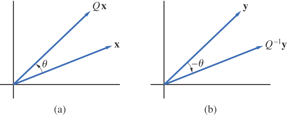
The matrix Q in Example 6 can be thought of as a linear transformation from R² onto R2 $ℝ^{2}$ that has the effect of rotating each vector by an angle θ $θ$ while leaving the length of the vector unchanged (see Example 2 in Section 4.2). Similarly, Q−1 $Q^{- 1}$ can be thought of as a rotation by the angle −θ $- θ$ (see Figure 5.5.1).

Two vector diagrams, a and b, have two vectors, each.

Figure 5.5.1. Full Alternative Text

In general, inner products are preserved under multiplication by an orthogonal matrix [i.e., ⟨x,y⟩=⟨Qx,Qy⟩ $〈 x, y 〉 = 〈 Q x, Q y 〉$ ]. Indeed,

⟨ Q x, Q y ⟩ = (Q y) T Q x = y T Q T x = y T x = ⟨ x, y ⟩

$〈 Q x, Q y 〉 = {(Q y)}^{T} Q x = y^{T} Q^{T} x = y^{T} x = 〈 x, y 〉$

In particular, if x=y $x = y$ , then ∥Qx∥2=∥x∥2 ${‖ Q x ‖}^{2} = {‖ x ‖}^{2}$ and hence ∥Qx∥=∥x∥ $‖ Q x ‖ = ‖ x ‖$ . Multiplication by an orthogonal matrix preserves the lengths of vectors.

Properties of Orthogonal Matrices

If Q is an n×n $n \times n$ orthogonal matrix, then

the column vectors of Q form an orthonormal basis for Rn $ℝ^{n}$
QTQ=I $Q^{T} Q = I$
QT=Q−1 $Q^{T} = Q^{- 1}$
⟨Qx,Qy⟩=⟨x,y⟩ $〈 Q x, Q y 〉 = 〈 x, y 〉$
∥Qx∥2=∥x∥2 ${‖ Q x ‖}_{2} = {‖ x ‖}_{2}$

Permutation Matrices

A permutation matrix is a matrix formed from the identity matrix by reordering its columns. Clearly, then, permutation matrices are orthogonal matrices. If P is the permutation matrix formed by reordering the columns of I in the order (k1,…,kn) $(k_{1}, …, k_{n})$ , then P=(ek1,…,ekn) $P = (e_{k 1}, …, e_{k n})$ . If A is an m×n $m \times n$ matrix, then

A P = (A e k 1, \dots, A e k n) = (a k 1, \dots, a k n)

$A P = (A e_{k 1}, …, A e_{k n}) = (a_{k 1}, …, a_{k n})$

Postmultiplication of A by P reorders the columns of A in the order (k1,…,kn) $(k_{1}, …, k_{n})$ . For example, if

A = [112233] and P = ⎡ ⎣ ⎢ 001100010 ⎤ ⎦ ⎥

$\begin{matrix} A = [\begin{matrix} 1 & 2 & 3 \\ 1 & 2 & 3 \end{matrix}] & \begin{matrix} and & P = [\begin{matrix} 0 & 1 & 0 \\ 0 & 0 & 1 \\ 1 & 0 & 0 \end{matrix}] \end{matrix} \end{matrix}$

then

A P = [331122]

$A P = [\begin{matrix} 3 & 1 & 2 \\ 3 & 1 & 2 \end{matrix}]$

Since P=(ek1,……,ekn) $P = (e_{k 1}, ……, e_{k n})$ is orthogonal, it follows that

P - 1 = P T ⎡ ⎣ ⎢ ⎢ e T k 1 ⋮ e T k n ⎤ ⎦ ⎥ ⎥

$P^{- 1} = P^{T} [\begin{matrix} e_{k 1}^{T} \\ ⋮ \\ e_{k n}^{T} \end{matrix}]$

The k1 $k_{1}$ column of PT $P^{T}$ will be e1 $e_{1}$ , the k2 $k_{2}$ column will be e2 $e_{2}$ , and so on. Thus, PT $P^{T}$ is a permutation matrix. The matrix PT $P^{T}$ can be formed directly from I by reordering its rows in the order (k1,k2,…,kn) $(k_{1}, k_{2}, …, k_{n})$ . In general, a permutation matrix can be formed from I by reordering either its rows or its columns.

If Q is the permutation matrix formed by reordering the rows of I in the order (k1,k2,…,kn) $(k_{1}, k_{2}, …, k_{n})$ and B is an n×r $n \times r$ matrix, then

Q B = ⎡ ⎣ ⎢ ⎢ ⎢ e T k 1 ⋮ e T k n ⎤ ⎦ ⎥ ⎥ ⎥ B = ⎡ ⎣ ⎢ ⎢ ⎢ e T k 1 B ⋮ e T k n B ⎤ ⎦ ⎥ ⎥ ⎥ = ⎡ ⎣ ⎢ ⎢ ⎢ ⎢ b \to k 1 ⋮ b \to k n ⎤ ⎦ ⎥ ⎥ ⎥ ⎥

$Q B = [\begin{matrix} e_{k_{1}}^{T} \\ ⋮ \\ e_{k_{n}}^{T} \end{matrix}] B = [\begin{matrix} e_{k_{1}}^{T} B \\ ⋮ \\ e_{k_{n}}^{T} B \end{matrix}] = [\begin{matrix} {\vec{b}}_{k_{1}} \\ ⋮ \\ {\vec{b}}_{k_{n}} \end{matrix}]$

Thus, QB is the matrix formed by reordering the rows of B in the order (k1,k2,…,kn) $(k_{1,} k_{2}, …, k_{n})$ . For example, if

Q = ⎡ ⎣ ⎢ 010001100 ⎤ ⎦ ⎥ and B = ⎡ ⎣ ⎢ 123123 ⎤ ⎦ ⎥

$\begin{matrix} Q = [\begin{matrix} 0 & 0 & 1 \\ 1 & 0 & 0 \\ 0 & 1 & 0 \end{matrix}] & \begin{matrix} and & B = [\begin{matrix} 1 & 1 \\ 2 & 2 \\ 3 & 3 \end{matrix}] \end{matrix} \end{matrix}$

then

Q B = ⎡ ⎣ ⎢ 312312 ⎤ ⎦ ⎥

$Q \begin{matrix} B = [\begin{matrix} 3 & 3 \\ 1 & 1 \\ 2 & 2 \end{matrix}] \end{matrix}$

In general, if P is an n×n $n \times n$ permutation matrix, premultiplication of an n×r $n \times r$ matrix B by P reorders the rows of B and postmultiplication of an m×n $m \times n$ matrix A by P reorders the columns of A.

Orthonormal Sets and Least Squares

Orthogonality plays an important role in solving least squares problems. Recall that if A is an m×n $m \times n$ matrix of rank n, then the least squares problem Ax=b $A x = b$ has a unique solution xˆ $\hat{x}$ that is determined by solving the normal equations ATAx=ATb $A^{T} A x = A^{T} b$ . The projection p=Axˆ $p = A \hat{x}$ is the vector in R(A) that is closest to b. The least squares problem is especially easy to solve in the case where the column vectors of A form an orthonormal set in Rm $ℝ^{m}$ .

Theorem 5.5.6

If the column vectors of A form an orthonormal set of vectors in Rm $ℝ^{m}$ , then ATA=I $A^{T} A = I$ and the solution to the least squares problem is

x ˆ = A T b

$\hat{x} = A^{T} b$

Proof

The (i, j) entry of ATA $A^{T} A$ is formed from the ith row of AT $A^{T}$ and the jth column of A. Thus, the (i, j) entry is actually the scalar product of the ith and jth columns of A. Since the column vectors of A are orthonormal, it follows that

A T A = (δ i j) = I

$A^{T} A = (δ_{i j}) = I$

Consequently, the normal equations simplify to

x = A T b

$x = A^{T} b$

∎

What if the columns of A are not orthonormal? In the next section, we will learn a method for finding an orthonormal basis for R(A). From this method, we will obtain a factorization of A into a product QR, where Q has an orthonormal set of column vectors and R is upper triangular. With this factorization, the least squares problem is easily solved.

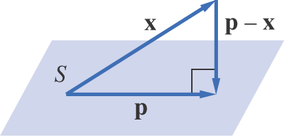
If we have an orthonormal basis for R(A), the projection p = Axˆ $\hat{x}$ can be determined in terms of the basis elements. Indeed, this is a special case of the more general least squares problem of finding the element p in a subspace S of an inner product space V that is closest to a given element x in V. This problem is easily solved if S has an orthonormal basis. We first prove the following theorem.

Theorem 5.5.7

Let S be a subspace of an inner product space V and let x∈V $x \in V$ . Let {u1,u2,,…,un} ${u_{1}, u_{2},, …, u_{n}}$ be an orthonormal basis for S. If

p = \sum i = 1 n c i u i

$p = \sum_{i = 1}^{n} c_{i} u_{i}$ (3)

where

c i = ⟨ x, u i ⟩ f o r e a c h i

$\begin{matrix} c_{i} = 〈 x, u_{i} 〉 & f o r e a c h i \end{matrix}$ (4)

then p−x∈S⊥ $p - x \in S^{⊥}$ (see Figure 5.5.2).

Three vectors form a right triangle on a plane, S.

Figure 5.5.2. Full Alternative Text

Proof

We will show first that (p−x)⊥ui $(p - x) ⊥ u_{i}$ for each i.

⟨ u i, p - x ⟩ = = = = ⟨ u i, p ⟩ - ⟨ u i, x ⟩ ⟨ u i, \sum j = 1 n c j u j ⟩ - c i \sum j = 1 n c j ⟨ u i, u j ⟩ - c i 0

$\begin{matrix} 〈 u_{i}, p - x 〉 & = & 〈 u_{i}, p 〉 - 〈 u_{i}, x 〉 \\ = & 〈 u_{i}, \sum_{j = 1}^{n} c_{j} u_{j} 〉 - c_{i} \\ = & \sum_{j = 1}^{n} c_{j} 〈 u_{i}, u_{j} 〉 - c_{i} \\ = & 0 \end{matrix}$

So p−x $p - x$ is orthogonal to all the ui's $u_{i}' s$ . If y∈S $y \in S$ , then

y = \sum i = 1 n α i u i

$y = \sum_{i = 1}^{n} α_{i} u_{i}$

and hence

⟨ p - x, y ⟩ = ⟨ p - x, \sum i = 1 n α i u i ⟩ = \sum i = 1 n α i ⟨ p - x, u i ⟩ = 0

$〈 p - x, y 〉 = 〈 p - x, \sum_{i = 1}^{n} α_{i} u_{i} 〉 = \sum_{i = 1}^{n} α_{i} 〈 p - x, u_{i} 〉 = 0$

∎

If x∈S $x \in S$ , the preceding result is trivial, since by Theorem 5.5.2, p−x=0 $p - x = 0$ . If x∉S $x \notin S$ , then p is the element in S closest to x.

Theorem 5.5.8

Under the hypothesis of Theorem 5.5.7, p is the element of S that is closest to x; that is,

∥ y - x ∥ > ∥ p - x ∥

$‖ y - x ‖ > ‖ p - x ‖$

for any y≠p $y \neq p$ in S.

Proof

If y∈S $y \in S$ and y≠p $y \neq p$ , then

∥ y - x ∥ 2 = ∥ (y - p) + (p - x) ∥ 2

${‖ y - x ‖}^{2} = {‖ (y - p) + (p - x) ‖}^{2}$

Since y−p∈S $y - p \in S$ , it follows from Theorem 5.5.7 and the Pythagorean law that

∥ y - x ∥ 2 = ∥ y - p ∥ 2 + ∥ p - x ∥ 2 > ∥ p - x ∥ 2

$‖ y - x ‖^{2} = {‖ y - p ‖}^{2} + {‖ p - x ‖}^{2} > {‖ p - x ‖}^{2}$

Therefore, ∥y−x∥>∥p−x∥ $‖ y - x ‖ > ‖ p - x ‖$ .

∎

The vector p defined by (3) and (4) is said to be the projection of x onto S.

Corollary 5.5.9

Let S be a nonzero subspace of Rm $ℝ^{m}$ and let b∈Rm $b \in ℝ^{m}$ . If {u1,u2,…,uk} ${u_{1}, u_{2}, …, u_{k}}$ is an orthonormal basis for S and U=(u1,u2,…,uk) $U = (u_{1}, u_{2}, …, u_{k})$ , then the projection p of b onto S is given by

p = U U T b

$p = U U^{T} b$

Proof

It follows from Theorem 5.5.7 that the projection p of b onto S is given by

p = c 1 u 1 + c 2 u 2 + \dots + c k u k = U c

$p = c_{1} u_{1} + c_{2} u_{2} + ⋯ + c_{k} u_{k} = U_{c}$

where

c = ⎡ ⎣ ⎢ ⎢ ⎢ ⎢ c 1 c 2 ⋮ c k ⎤ ⎦ ⎥ ⎥ ⎥ ⎥ = ⎡ ⎣ ⎢ ⎢ ⎢ ⎢ ⎢ u T 1 b u T 2 b ⋮ u T k b ⎤ ⎦ ⎥ ⎥ ⎥ ⎥ ⎥ = U T b

$c = [\begin{matrix} c_{1} \\ c_{2} \\ ⋮ \\ c_{k} \end{matrix}] = [\begin{matrix} u_{1}^{T} b \\ u_{2}^{T} b \\ ⋮ \\ u_{k}^{T} b \end{matrix}] = U^{T} b$

Therefore,

p = U U T b

$p = U U^{T} b$

∎

The matrix UUT $U U^{T}$ in Corollary 5.5.9 is the projection matrix corresponding to the subspace S of Rm $ℝ^{m}$ . To project any vector b∈Rm $b \in ℝ^{m}$ onto S, we need only find an orthonormal basis {u1,u2,…,uk} ${u_{1}, u_{2}, …, u_{k}}$ for S, form the matrix UUT $U U^{T}$ , and then multiply UUT $U U^{T}$ times b.

If P is a projection matrix corresponding to a subspace S of Rm $ℝ^{m}$ , then, for any b∈Rm $b \in ℝ^{m}$ , the projection p of b onto S is unique. If Q is also a projection matrix corresponding to S, then

Q b = p = P b

$Q b = p = P b$

It then follows that

q j = Q e j = P e j = P e j = p j for j = 1, \dots, m

$\begin{matrix} q_{j} = Q e_{j} = P e_{j} = P e_{j} = p_{j} & for j = 1, …, m \end{matrix}$

and hence Q=P $Q = P$ . Thus, the projection matrix for a subspace S of Rm $ℝ^{m}$ is unique.

Example 7

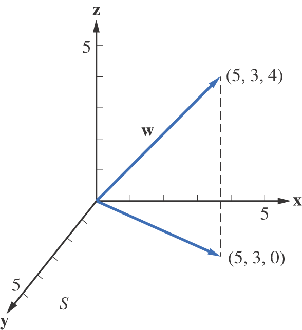
Let S be the set of all vectors in R3 $ℝ^{3}$ of the form (x,y,0)T ${(x, y, 0)}^{T}$ . Find the vector p in S that is closest to w=(5,3,4)T $w = {(5, 3, 4)}^{T}$ (see Figure 5.5.3).

The graph of x y z plane has two vectors rising from the origin. Vector w rises from the origin to the terminal point (5, 3, 4). The other vector falls from the origin to the terminal point (5, 3, 0). A dotted line is drawn from (5, 3, 4) to (5, 3, 0).

Figure 5.5.3. Full Alternative Text

SOLUTION

Let u1=(1,0,0)T $u_{1} = {(1, 0, 0)}^{T}$ and u2=(0,1,0)T $u_{2} = {(0, 1, 0)}^{T}$ . Clearly, u1 $u_{1}$ and u2 $u_{2}$ form an orthonormal basis for S. Now

c 1 c 2 = = w T u 1 = 5 w T u 2 = 3

$\begin{matrix} c_{1} & = & w^{T} u_{1} = 5 \\ c_{2} & = & w^{T} u_{2} = 3 \end{matrix}$

The vector p turns out to be exactly what we would expect:

p = 5 u 1 + 3 u 2 = (5, 3, 0) T

$p = 5 u_{1} + 3 u_{2} = {(5, 3, 0)}^{T}$

Alternatively, p could have been calculated using the projection matrix UUT $U U^{T}$ .

p = U U T w = ⎡ ⎣ ⎢ 100010000 ⎤ ⎦ ⎥ ⎡ ⎣ ⎢ 534 ⎤ ⎦ ⎥ = ⎡ ⎣ ⎢ 530 ⎤ ⎦ ⎥

$p = U U^{T} w = [\begin{matrix} 1 & 0 & 0 \\ 0 & 1 & 0 \\ 0 & 0 & 0 \end{matrix}] [\begin{matrix} 5 \\ 3 \\ 4 \end{matrix}] = [\begin{matrix} 5 \\ 3 \\ 0 \end{matrix}]$

Approximation of Functions

In many applications, it is necessary to approximate a continuous function in terms of functions from some special type of approximating set. Most commonly, we approximate by a polynomial of degree n or less. We can use Theorem 5.5.8 to obtain the best least squares approximation.

Example 8

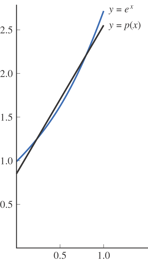
Find the best least squares approximation to ex $e^{x}$ on the interval [0, 1] by a linear function.

SOLUTION

Let S be the subspace of all linear functions in C[0, 1]. Although the functions 1 and x span S, they are not orthogonal. We seek a function of the form x−a $x - a$ that is orthogonal to 1.

⟨ 1, x - a ⟩ = \int 10 (x - a) d x = 1 2 - a

$〈 1, x - a 〉 = \int_{0}^{1} (x - a) d x = \frac{1}{2} - a$

Thus, a=12 $a = \frac{1}{2}$ . Since ∥∥x−12∥∥=1/12−−√ $‖ x - \frac{1}{2} ‖ = 1 / \sqrt{12}$ , it follows that

u 1 (x) = 1 and u 2 (x) = 12 - - \sqrt (x - 1 2)

$\begin{matrix} u_{1} (x) = 1 & \begin{matrix} \begin{matrix} and \end{matrix} & u_{2} (x) = \sqrt{12} (x - \frac{1}{2}) \end{matrix} \end{matrix}$

form an orthonormal basis for S.

Let

c 1 c 2 = = \int 10 u 1 (x) e x d x = e - 1 \int 10 u 2 (x) e x d x = 3 - \sqrt (3 - e)

$\begin{matrix} c_{1} & = & \int_{0}^{1} u_{1} (x) e^{x} d x = e - 1 \\ c_{2} & = & \int_{0}^{1} u_{2} (x) e^{x} d x = \sqrt{3} (3 - e) \end{matrix}$

The projection

P (x) = = = c 1 u 1 (x) + c 2 u 1 (x) (e - 1) \cdot 1 + 3 - \sqrt (3 - e) [12 - - \sqrt (x - 1 2)] (4 e - 10) + 6 (3 - e) x

$\begin{matrix} P (x) & = & c_{1} u_{1} (x) + c_{2} u_{1} (x) \\ = & (e - 1) \cdot 1 + \sqrt{3} (3 - e) [\sqrt{12} (x - \frac{1}{2})] \\ = & (4 e - 10) + 6 (3 - e) x \end{matrix}$

is the best linear least squares approximation to ex $e^{x}$ on [0, 1] (see Figure 5.5.4).

A graph plots a concave up increasing curve, y = e to the x power, that rises from (0, 1.0) to (1.0, 2.9). A tangent line, y = p of x, rises from (0, 0.9) to (1.1, 2.6). All values estimated.

Figure 5.5.4. Full Alternative Text

Approximation by Trigonometric Polynomials

Trigonometric polynomials are used to approximate periodic functions. By a trigonometric polynomial of degree n, we mean a function of the form

t n (x) = a 0 2 + \sum k = 1 n (a k cos k x + b k sin k x)

$t_{n} (x) = \frac{a_{0}}{2} + \sum_{k = 1}^{n} (a_{k} \cos k x + b_{k} \sin k x)$

We have already seen that the collection of functions

1 2 - \sqrt, cos x, cos 2 x, \dots, cos n x

$\frac{1}{\sqrt{2}}, \cos x, \cos 2 x, …, \cos n x$

forms an orthonormal set with respect to the inner product (2). We leave it to the reader to verify that if the functions

sin x, sin 2 x, \dots, sin n x

$\sin x, \sin 2 x, …, \sin n x$

are added to the collection, it will still be an orthonormal set. Thus, we can use Theorem 5.5.8 to find the best least squares approximation to a continuous 2π periodic function f (x) by a trigonometric polynomial of degree n or less. Note that

⟨ f, 1 2 - \sqrt ⟩ 1 2 - \sqrt = ⟨ f, 1 ⟩ 1 2

$〈 f, \frac{1}{\sqrt{2}} 〉 \frac{1}{\sqrt{2}} = 〈 f, 1 〉 \frac{1}{2}$

so that if

a 0 = ⟨ f, 1 ⟩ = 1 π \int π - π f (x) d x

$a_{0} = 〈 f, 1 〉 = \frac{1}{π} \int_{- π}^{π} f (x) d x$

and

a k b k = = ⟨ f, cos k x ⟩ = 1 π \int π - π f (x) cos k x d x ⟨ f, sin k x ⟩ = 1 π \int π - π f (x) sin k x d x

$\begin{matrix} a_{k} & = & 〈 f, \cos k x 〉 = \frac{1}{π} \int_{- π}^{π} f (x) \cos k x d x \\ b_{k} & = & 〈 f, \sin k x 〉 = \frac{1}{π} \int_{- π}^{π} f (x) \sin k x d x \end{matrix}$

for k=1,2,…,n $k = 1, 2, …, n$ , then these coefficients determine the best least squares approximation to f. The ak’s $a_{k} ’s$ and the bk’s $b_{k} ’s$ turn out to be the well-known Fourier coefficients that occur in many applications involving trigonometric series approximations of functions.

Let us think of f (x) as representing the position at time x of an object moving along a line, and let tn $t_{n}$ be the Fourier approximation of degree n to f. If we set

r k = a 2 k + b 2 k - - - - - - \sqrt and θ k = Tan - 1 (b k a k)

$\begin{matrix} r_{k} = \sqrt{a_{k}^{2} + b_{k}^{2}} & \begin{matrix} and & θ_{k} = {Tan}^{- 1} (\frac{b_{k}}{a_{k}}) \end{matrix} \end{matrix}$

then

a k cos k x + b k sin k x = = r k (a k r k cos k x + b k r k sin k x) r k cos (k x - θ k)

$\begin{matrix} a_{k} \cos k x + b_{k} \sin k x & = & r_{k} (\frac{a_{k}}{r_{k}} \cos k x + \frac{b_{k}}{r_{k}} \sin k x) \\ = & r_{k} \cos (k x - θ_{k}) \end{matrix}$

Thus, the motion f (x) is being represented as a sum of simple harmonic motions.

For signal-processing applications, it is useful to express the trigonometric approximation in complex form. To this end, we define complex Fourier coefficients ck $c_{k}$ in terms of the real Fourier coefficients ak $a_{k}$ and bk $b_{k}$ :

c k = 1 2 (a k - i b k) = = 1 2 π \int π - π f (x) (cos k x - i sin k x) d x 1 2 π \int π - π f (x) e - k x d x (k \geq 0)

$\begin{matrix} c_{k} = \frac{1}{2} (a_{k} - i b_{k}) & = & \frac{1}{2 π} \int_{- π}^{π} f (x) (\cos k x - i \sin k x) d x \\ = & \frac{1}{2 π} \int_{- π}^{π} f (x) e^{- k x} d x (k \geq 0) \end{matrix}$

The latter equality follows from the identity

e i θ = cos θ + i sin θ

$e^{i θ} = \cos θ + i \sin θ$

We also define the coefficient C−k $C_{- k}$ to be the complex conjugate of Ck $C_{k}$ . Thus,

C - k = C k ¯ ¯ ¯ ¯ = 1 2 (a k + i b k) (k \geq 0)

$\begin{matrix} C_{- k} = \bar{C_{k}} = \frac{1}{2} (a_{k} + i b_{k}) & (k \geq 0) \end{matrix}$

Alternatively, if we solve for ak $a_{k}$ and bk $b_{k}$ , then

a k = c k + c - k and b k = i (c k - c - k)

$\begin{matrix} a_{k} = c_{k} + c_{- k} & \begin{matrix} and & b_{k} = i (c_{k} - c_{- k}) \end{matrix} \end{matrix}$

From these identities, it follows that

c k e - k x + c - k e - i k x = = (c k + c - k) cos k x + i (c k - c - k) sin k x a k cos k x + b k sin k x

$\begin{matrix} c_{k} e^{- k x} + c_{- k} e^{- i k x} & = & (c_{k} + c_{- k}) \cos k x + i (c_{k} - c_{- k}) \sin k x \\ = & a_{k} \cos k x + b_{k} \sin k x \end{matrix}$

and hence the trigonometric polynomial

t n (x) = a 0 2 + \sum k = 1 n (a k cos k x + b k sin k x)

$t_{n} (x) = \frac{a_{0}}{2} + \sum_{k = 1}^{n} (a_{k} \cos k x + b_{k} \sin k x)$

can be rewritten in complex form as

t n (x) = \sum k = - n n c k e i k x

$t_{n} (x) = \sum_{k = - n}^{n} c_{k} e^{i k x}$

Application 1

Signal Processing

The Discrete Fourier Transform

The function f (x) pictured in Figure 5.5.5(a) corresponds to a noisy signal. Here, the independent variable x represents time and the signal values are plotted as a function of time. In this context, it is convenient to start with time 0. Thus, we will choose [0, 2π], rather than [−π,π] $[- π, π]$ , as the interval for our inner product.

Figure 5.5.5.

Figure 5.5.5. Full Alternative Text

Let us approximate f (x) by a trigonometric polynomial

t n (x) = \sum k = - n n c k e i k x

$t_{n} (x) = \sum_{k = - n}^{n} c_{k} e^{i k x}$

As noted in the previous discussion, the trigonometric approximation allows us to represent the function as a sum of simple harmonics. The kth harmonic can be written as rkcos(kx−θk) $r_{k} \cos (kx - θ_{k})$ . It is said to have angular frequency k. A signal is smooth if the coefficients ck $c_{k}$ approach 0 rapidly as k increases. If some of the coefficients corresponding to larger frequencies are not small, the graph will appear to be noisy as in Figure 5.5.5(a). We can filter the signal by setting these coefficients equal to 0. Figure 5.5.5(b) shows the smooth function obtained by suppressing some of the higher frequencies from the original signal.

In actual signal-processing applications, we do not have a mathematical formula for the signal function f (x); rather, the signal is sampled over a sequence of times x0,x1,…,xN $x_{0}, x_{1}, …, x_{N}$ , where xj=2jπN $x_{j} = \frac{2 j π}{N}$ . The function f is represented by the N sample values

y 0 = f (x 0), y 1 = f (x 1), \dots, y N - 1 = f (x N - 1)

$y_{0} = f (x_{0}), y_{1} = f (x_{1}), …, y_{N - 1} = f (x_{N - 1})$

[Note: yN=f(2π)=f(0)=y0 $y_{N} = f (2 π) = f (0) = y_{0}$ .] In this case, it is not possible to compute the Fourier coefficients as integrals. Instead of using

c k = 1 2 π \int 2 π 0 f (x) e - i k x d x

$c_{k} = \frac{1}{2 π} \int_{0}^{2 π} f (x) e^{- ikx} d x$

we use a numerical integration method, the trapezoid rule, to approximate the integral. The approximation is given by

d k = 1 N \sum j = 0 N - 1 f (x j) e - i k x j

$d_{k} = \frac{1}{N} \sum_{j = 0}^{N - 1} f (x_{j}) e^{- i k x_{j}}$ (5)

The dk $d_{k}$ coefficients are approximations to the Fourier coefficients. The larger the sample size N, the closer dk $d_{k}$ will be to ck $c_{k}$ .

If we set

ω N = e - 2 π i N = cos 2 π N - i sin 2 π N

$ω_{N} = e^{- \frac{2 π i}{N}} = \cos \frac{2 π}{N} - i \sin \frac{2 π}{N}$

then equation (5) can be rewritten in the form

d k = 1 N \sum j = 0 N - 1 y j ω j k N

$d_{k} = \frac{1}{N} \sum_{j = 0}^{N - 1} y_{j} ω_{N}^{j k}$

The finite sequence {d0,d1,…,dN−1} ${d_{0}, d_{1}, …, d_{N - 1}}$ is said to be the discrete Fourier transform of {y0,y1,…,yN−1} ${y_{0}, y_{1}, …, y_{N - 1}}$ . The discrete Fourier transform can be determined by a single matrix vector multiplication. For example, if N=4 $N = 4$ , the coefficients are given by

d 0 d 1 d 2 d 3 = 1 4 (y 0 + y 1 + y 2 + y 3) = 1 4 (y 0 + ω 4 y 1 + ω 24 y 2 + ω 34 y 3) = 1 4 (y 0 + w 24 y 1 + ω 44 y 2 + ω 64 y 3) = 1 4 (y 0 + ω 34 y 1 + ω 64 y 2 + ω 94 y 4)

$\begin{matrix} d_{0} & \begin{matrix} \begin{matrix} = \end{matrix} & \frac{1}{4} (y_{0} + y_{1} + y_{2} + y_{3}) \end{matrix} \\ d_{1} & \begin{matrix} \begin{matrix} = \end{matrix} & \frac{1}{4} (y_{0} + ω_{4} y_{1} + ω_{4}^{2} y_{2} + ω_{4}^{3} y_{3}) \end{matrix} \\ d_{2} & \begin{matrix} \begin{matrix} = \end{matrix} & \frac{1}{4} (y_{0} + w_{4}^{2} y_{1} + ω_{4}^{4} y_{2} + ω_{4}^{6} y_{3}) \end{matrix} \\ d_{3} & \begin{matrix} \begin{matrix} = \end{matrix} & \frac{1}{4} (y_{0} + ω_{4}^{3} y_{1} + ω_{4}^{6} y_{2} + ω_{4}^{9} y_{4}) \end{matrix} \end{matrix}$

If we set

z = 1 4 y = 1 4 (y 0, y 1, y 3) T

$z = \frac{1}{4} y = \frac{1}{4} {(y_{0}, y_{1}, y_{3})}^{T}$

then the vector d=(d0,d1,d2,d3)T $d = {(d_{0}, d_{1}, d_{2}, d_{3})}^{T}$ is determined by multiplying z by the matrix

F 4 = ⎡ ⎣ ⎢ ⎢ ⎢ ⎢ 1111 1 ω 4 ω 24 ω 43 1 ω 24 ω 44 ω 64 1 ω 34 ω 46 ω 94 ⎤ ⎦ ⎥ ⎥ ⎥ ⎥ = ⎡ ⎣ ⎢ ⎢ ⎢ ⎢ 1111 1 - i - 1 i 1 - 1 1 - 1 1 i - 1 - i ⎤ ⎦ ⎥ ⎥ ⎥ ⎥

$F_{4} = [\begin{matrix} 1 & 1 & 1 & 1 \\ 1 & ω_{4} & ω_{4}^{2} & ω_{4}^{3} \\ 1 & ω_{4}^{2} & ω_{4}^{4} & ω_{6}^{4} \\ 1 & ω_{3}^{4} & ω_{4}^{6} & ω_{4}^{9} \end{matrix}] = [\begin{matrix} 1 & 1 & 1 & 1 \\ 1 & - i & - 1 & i \\ 1 & - 1 & 1 & - 1 \\ 1 & i & - 1 & - i \end{matrix}]$

The matrix F4 $F_{4}$ is called a Fourier matrix.

In the case of N sample values, y0,y1,…,yN−1 $y_{0}, y_{1}, …, y_{N - 1}$ , the coefficients are computed by setting

z = 1 N y and d = F N z

$\begin{matrix} z = \frac{1}{N} y & \begin{matrix} and & d = F_{N} z \end{matrix} \end{matrix}$

where y=(y0,y1,…,yN−1)T $y = {(y_{0}, y_{1}, …, y_{N - 1})}^{T}$ and FN $F_{N}$ is the N×N $N \times N$ matrix whose (j, k) entry is given by fj,k=ω(j−1)(k−1)N $f_{j, k} = ω_{N}^{(j - 1) (k - 1)}$ . The method of computing the discrete Fourier transform d by multiplying FN $F_{N}$ times z will be referred to as the DFT algorithm. The DFT computation requires a multiple of N2 $N^{2}$ arithmetic operations (roughly 8N2 $8 N^{2}$ , since complex arithmetic is used).

In signal-processing applications, N is generally very large and consequently the DFT computation of the discrete Fourier transform can be prohibitively slow and costly even on modern high-powered computers. A revolution in signal processing occurred in 1965 with the introduction by James W. Cooley and John W. Tukey of a dramatically more efficient method for computing the discrete Fourier transform. Actually, it turns out that the 1965 Cooley–Tukey paper is a rediscovery of a method that was known to Gauss in 1805.

The Fast Fourier Transform

The method of Cooley and Tukey, known as the fast Fourier transform or simply the FFT, is an efficient algorithm for computing the discrete Fourier transform. It takes advantage of the special structure of the Fourier matrices. We illustrate this method in the case N=4 $N = 4$ . To see the special structure, we rearrange the columns of F4 $F_{4}$ so that its odd-numbered columns all come before the even-numbered columns. This rearrangement is equivalent to postmultiplying F4 $F_{4}$ by the permutation matrix

P 4 = ⎡ ⎣ ⎢ ⎢ ⎢ ⎢ 1000001001000001 ⎤ ⎦ ⎥ ⎥ ⎥ ⎥

$P_{4} = [\begin{matrix} 1 & 0 & 0 & 0 \\ 0 & 0 & 1 & 0 \\ 0 & 1 & 0 & 0 \\ 0 & 0 & 0 & 1 \end{matrix}]$

If we set w=PT4z $w = P_{4}^{T} z$ , then

F 4 z = F 4 P 4 P T 4 z = F 4 P 4 w

$F_{4} z = F_{4} P_{4} P_{4}^{T} z = F_{4} P_{4} w$

Partitioning F4P4 $F_{4} P_{4}$ into 2×2 $2 \times 2$ blocks, we get

5.9-6 Full Alternative Text

The (1,1) and (2,1) blocks are both equal to the Fourier matrix F2 $F_{2}$ , and if we set

D 2 = [10 - 0 - i]

$D_{2} = [\begin{matrix} 1 & 0 \\ 0 & - i \end{matrix}]$

then the (1,2) and (2,2) blocks are D2F2 $D_{2} F_{2}$ and −D2F2 $- D_{2} F_{2}$ , respectively. The computation of the Fourier transform can now be carried out as a block multiplication.

d 4 = [F 2 F 2 D 2 F 2 - D 2 F 2] [w 1 w 2] = [F 2 w 1 + D 2 F 2 w 2 F 2 w 1 - D 2 F 2 w 2]

$d_{4} = [\begin{matrix} F_{2} & D_{2} F_{2} \\ F_{2} & - D_{2} F_{2} \end{matrix}] [\begin{matrix} w_{1} \\ w_{2} \end{matrix}] = [\begin{matrix} F_{2} w_{1} + D_{2} F_{2} w_{2} \\ F_{2} w_{1} - D_{2} F_{2} w_{2} \end{matrix}]$

The computation reduces to computing two Fourier transforms of length 2. If we set q1=F2w1 $q_{1} = F_{2} w_{1}$ and q2=D2(F2w2) $q_{2} = D_{2} (F_{2} w_{2})$ , then

d 4 = [q 1 + q 2 q 1 + q 2]

$d_{4} = [\begin{matrix} q_{1} + q_{2} \\ q_{1} + q_{2} \end{matrix}]$

The procedure we have just described will work in general whenever the number of sample points is even. If, say, N=2m $N = 2 m$ , and we permute the columns of F2m $F_{2 m}$ so that the odd columns are first, then the reordered Fourier matrix F2mP2m $F_{2 m} P_{2 m}$ can be partitioned into m×m $m \times m$ blocks

F 2 m P 2 m = [F m F m D m F m - D m F m]

$F_{2 m} P_{2 m} = [\begin{matrix} F_{m} & D_{m} F_{m} \\ F_{m} & - D_{m} F_{m} \end{matrix}]$

where Dm $D_{m}$ is a diagonal matrix whose (j, j) entry is ωj−i2m $ω_{2 m}^{j - i}$ . The discrete Fourier transform can then be computed in terms of two transforms of length m. Furthermore, if m is even, then each length m transform can be computed in terms of two transforms of length m2 $\frac{m}{2}$ , and so on.

If, initially, N is a power of 2, say, N=2k $N = 2^{k}$ , then we can apply this procedure recursively through k levels of recursion. The amount of arithmetic required to compute the FFT is proportional to Nk=N log2N $N k = N \log_{2} N$ . In fact, the actual amount of arithmetic operations required for the FFT is approximately 5N log2N $5 N \log_{2} N$ . How dramatic of a speedup is this? If we consider, for example, the case where N=220=1,048.576 $N = 2^{20} = 1, 048.576$ , then the DFT algorithm requires 8N2=8⋅240 $8 N^{2} = 8 \cdot 2^{40}$ operations, that is, approximately 8.8 trillion operations. On the other hand, the FFT algorithm requires only 100N=100⋅220 $100 N = 100 \cdot 2^{20}$ , or approximately 100 million, operations. The ratio of these two operations counts is

r = 8 N 2 5 N log 2 N = 0.08 \cdot 1,048,576 = 83, 886

$r = \frac{8 N^{2}}{5 N \log_{2} N} = 0.08 \cdot 1,048,576 = 83, 886$

In this case, the FFT algorithm is approximately 84,000 times faster than the DFT algorithm.

..................Content has been hidden....................

You can't read the all page of ebook, please click here login for view all page.

Table of Contents for 5.5 Orthonormal Sets

Create new playlist

Sign In

Sign Up

Table of Contents for
5.5 Orthonormal Sets