In many applications, it is necessary either to determine the rank of a matrix or to determine whether the matrix is deficient in rank. Theoretically, we can use Gaussian elimination to reduce the matrix to row echelon form and then count the number of nonzero rows. However, this approach is not practical in finite-precision arithmetic. If A is rank deficient and U is the computed echelon form, then, because of rounding errors in the elimination process, it is unlikely that U will have the proper number of nonzero rows. In practice, the coefficient matrix A usually involves some error. This may be due to errors in the data or to the finite number system. Thus, it is generally more practical to ask whether A is “close” to a rank-deficient matrix. However, it may well turn out that A is close to being rank deficient and the computed row echelon form U is not.

In this section, we assume throughout that A is an $m\times n$ matrix with $m\ge n$. (This assumption is made for convenience only; all the results will also hold if $m<n$.) We will present a method for determining how close A is to a matrix of smaller rank. The method involves factoring A into a product $U\mathrm{\Sigma }{V}^T$, where U is an $m\times m$ orthogonal matrix, V is an $n\times n$ orthogonal matrix, and $\mathrm{\Sigma }$ is an $m\times n$ matrix whose off-diagonal entries are all 0’s and whose diagonal elements satisfy

The ${\sigma }_i$’s determined by this factorization are unique and are called the singular values of A. The factorization $U\mathrm{\sum }{V}^T$ is called the singular value decomposition of A, or, for short, the svd of A. We will show that the rank of A equals the number of nonzero singular values, and that the magnitudes of the nonzero singular values provide a measure of how close A is to a matrix of lower rank.

We begin by showing that such a decomposition is always possible.

Proof

$A^{T}A$ is a symmetric $n\times n$ matrix. Therefore, its eigenvalues are all real and it has an orthogonal diagonalizing matrix V. Furthermore, its eigenvalues must all be nonnegative. To see this, let $\lambda$ be an eigenvalue of $A^{T}A$ and x be an eigenvector belonging to $\lambda$. It follows that

Hence,

We may assume that the columns of V have been ordered so that the corresponding eigenvalues satisfy

The singular values of A are given by

Let r denote the rank of A. The matrix $A^{T}A$ will also have rank r. Since $A^{T}A$ is symmetric, its rank equals the number of nonzero eigenvalues. Thus,

The same relation holds for the singular values

Now let

and

Hence, ${\mathrm{\sum }}_1$ is an $r\times r$ diagonal matrix whose diagonal entries are the nonzero singular values ${\sigma }_1,\mathrm{\dots },{\sigma }_r$. The $m\times n$ matrix $\mathrm{\sum }$ is then given by

The column vectors of $V_2$ are eigenvectors of $A^{T}A$ belonging to $\lambda =0$. Thus,

and, consequently, the column vectors of $V_2$ form an orthonormal basis for $N\left(A^{T}A\right)=N\left(A\right)$. Therefore,

and since V is an orthogonal matrix, it follows that

So far we have shown how to construct the matrices V and Σ of the singular value decomposition. To complete the proof, we must show how to construct an $m\times m$ orthogonal matrix U such that

or, equivalently,

Comparing the first r columns of each side of (3), we see that

Thus, if we define

and

then it follows that

The column vectors of $U_1$ form an orthonormal set since

It follows from (4) that each ${\mathbf{u}}_j,1\le j\le r$, is in the column space of A. The dimension of the column space is r, so ${\mathbf{u}}_1,\mathrm{\dots },{\mathbf{u}}_r$ form an orthonormal basis for $R\left(A\right)$. The vector space ${R\left(A\right)}^{\perp }=N\left(A^T\right)$ has dimension $m-r$. Let $\{{\mathbf{u}}_{r+1},{\mathbf{u}}_{r+2},\mathrm{\dots },{\mathbf{u}}_m\}$ be an orthonormal basis for $N\left(A^T\right)$ and set

It follows from Theorem 5.2.2 that ${\mathbf{u}}_1,\mathrm{\dots },{\mathbf{u}}_m$ form an orthonormal basis for ${ℝ}^m$. Hence, U is an orthogonal matrix. We still must show that $U\mathrm{\Sigma }{V}^T$ actually equals A. This follows from (5) and (2) since

∎

Visualizing the SVD

If we view an $m\times n$ matrix A with rank r as a mapping from the row space of A to the column space of A, then in light of observations (4) and (5) made earlier, it seems natural to choose ${\mathbf{v}}_1,{\mathbf{v}}_2,\dots ,{\mathbf{v}}_r$ as an orthonormal basis for the row space, since the image vectors

$$A{\mathbf{v}}_1={\sigma }_1{\mathbf{u}}_1,A{\mathbf{v}}_2={\sigma }_2{\mathbf{u}}_2,\dots ,{A{\mathbf{v}}_r=\sigma }_r{\mathbf{u}}_r$$

are mutually orthogonal and the corresponding unit vectors ${\mathbf{u}}_1,{\mathbf{u}}_2,\dots ,{\mathbf{u}}_r$ will form an orthonormal basis for the column space of A. In the case of a $2\times 2$ matrix, the following example illustrates geometrically how one could search for the right singular vectors by moving around the unit circle.

Example 2

Let

$$A=\left[\begin{array}{cc}0.4& \hfill -0.3\\ 0.9& \hfill 1.2\end{array}\right]$$

To find a pair of right singular vectors of A, we must find a pair of orthonormal vectors x and y for which the image vectors Ax and Ay are orthogonal. Choosing the standard basis vectors for ${ℝ}^2$ does not work, for if $\mathbf{x}={\mathbf{e}}_1$ and $\mathbf{y}={\mathbf{e}}_2$, then the image vectors

$$\begin{array}{ccc}A{\mathbf{e}}_1={\mathbf{a}}_1=\left[\begin{array}{c}0.4\\ 0.9\end{array}\right]& \text{and}& A{\mathbf{e}}_2={\mathbf{a}}_2=\left[\begin{array}{c}-0.3\\ \hfill 1.2\end{array}\right]\end{array}$$

are not orthogonal. See Figure 6.5.1.

Figure 6.5.1.

Figure 6.5.1. Full Alternative Text

One way to search for the right singular vectors is to simultaneously rotate this initial pair of vectors around the unit circle and for each rotated pair

$$\begin{array}{cc}{\mathbf{x}}_1=\left[\begin{array}{c}\text{cos }t\\ \sin t\end{array}\right],& \mathbf{y}=\left[\begin{array}{c}-\sin t\\ \hfill \text{cos }t\end{array}\right]\end{array}$$

check to see if Ax and Ay are orthogonal. For the given matrix A, this will happen when the tip of our initial x vector gets rotated to the point (0.6,0.8). It follows that the right singular vectors are

$$\begin{array}{cc}{\mathbf{v}}_1=\left[\begin{array}{c}0.6\\ 0.8\end{array}\right],& {\mathbf{v}}_2=\left[\begin{array}{c}-0.8\\ \hfill 0.6\end{array}\right]\end{array}$$

Since

$$\begin{array}{cc}A{\mathbf{v}}_1=\left[\begin{array}{r}0\\ 1.5\end{array}\right]=1.5{\mathbf{e}}_2,& \begin{array}{cc}\begin{array}{c}\text{and}\end{array}& A{\mathbf{v}}_2=\left[\begin{array}{r}-0.5\\ 0\end{array}\right]=-0.5{\mathbf{e}}_1\end{array}\end{array}$$

it follows that the singular values are ${\sigma }_1=1.5$ and ${\sigma }_2=0.5$, and the left singular vectors are ${\mathbf{u}}_1={\mathbf{e}}_2$ and ${\mathbf{u}}_2={-\mathbf{e}}_1$. See Figure 6.5.2.

∎

Figure 6.5.2.

Figure 6.5.2. Full Alternative Text

Numerical Rank and Lower Rank Approximations

If A is an $m\times n$ matrix of rank r and $0<k<r$, we can use the singular value decomposition to find a matrix in ${ℝ}^{m\times n}$ of rank k that is closest to A with respect to the Frobenius norm. Let ? be the set of all $m\times n$ matrices of rank k or less. It can be shown that there is a matrix X in ? such that

$${\Vert A-X\Vert }_F=\underset{S\in ?}{\text{min}}\Vert A-{S\Vert }_F$$ (7)

We will not prove this result, since the proof is beyond the scope of this text. Assuming that the minimum is achieved, we will show how such a matrix X can be derived from the singular value decomposition of A. The following lemma will be useful.

Lemma 6.5.2

If A is an $m\times n$ matrix and Q is an $m\times m$ orthogonal matrix, then

$${\Vert QA\Vert }_F=\Vert A{\Vert }_F$$

Proof

$$\begin{array}{cc}\hfill {\Vert QA\Vert }_F^2& =\Vert (Q{\mathbf{a}}_1,Q{\mathbf{a}}_2,\dots ,Q{\mathbf{a}}_n){\Vert }_F^2\hfill \\ \hfill & =\mathrm{\sum }_{i=1}^n\Vert Q{{\mathbf{a}}_i\Vert }_2^2\hfill \\ \hfill & =\mathrm{\sum }_{i=1}^n\Vert {{\mathbf{a}}_i\Vert }_2^2\hfill \\ \hfill & {\begin{array}{c}=\Vert A\Vert \end{array}}_F^2\hfill \end{array}$$

∎

If A has singular value decomposition $U\mathrm{\Sigma }{V}^T$, then it follows from the lemma that

$$\Vert A{\Vert }_F=\Vert \mathrm{\Sigma }{V}^T{\Vert }_F$$

Since

$$\Vert \mathrm{\Sigma }{V}^T{\Vert }_F=\Vert (\mathrm{\Sigma }{V}^T{)}^T{\Vert }_F=\Vert {V\mathrm{\Sigma }}^T{\Vert }_F=\Vert {\mathrm{\Sigma }}^T{\Vert }_F$$

It follows that

$$\Vert A{\Vert }_F=({\sigma }_1^2+{\sigma }_2^2+\dots +{\sigma }_n^2{)}^{1/2}$$

Theorem 6.5.3

Let $A=U\mathrm{\Sigma }{V}^T$ be an $m\times n$ matrix, and let ? denote the set of all $m\times n$ matrices of rank k or less, where $0<k<\text{rank }\left(A\right)$. If X is a matrix in ? satisfying (7), then

$$\Vert A-X{\Vert }_F=({\sigma }_{k+1}^2+{\sigma }_{k+2}^2+\dots +{\sigma }_n^2{)}^{1/2}$$

In particular, if $A^{\prime }=U{\mathrm{\Sigma }}^{\prime }{V}^T$, where

then

$$\Vert A-A^{\prime }{\Vert }_F=({\sigma }_{k+1}^2+\dots +{\sigma }_n^2{)}^{1/2}=\underset{S\in \mathcal{M}}{\text{min}}\Vert A-S{\Vert }_F$$

Proof

Let X be a matrix in M satisfying (7). Since $A^{\prime }\in ?$, it follows that

$$\Vert A-X{\Vert }_F\le {\Vert A-A^{\prime }\Vert }_F=({\sigma }_{k+1}^2+\dots +{\sigma }_n^2{)}^{1/2}$$ (8)

We will show that

$$\Vert A-X{\Vert }_F\ge =({\sigma }_{k+1}^2+\dots +{\sigma }_n^2{)}^{1/2}$$

and hence that equality holds in (8). Let $Q\mathrm{\Omega }{P}^T$ be the singular value decomposition of X, where

If we set $B=Q^{T}AP$, then $A={QBP}^T$, and it follows that

$$\Vert A-X{\Vert }_F=\Vert Q(B-\mathrm{\Omega })P^T{\Vert }_F=\Vert B-\mathrm{\Omega }{\Vert }_F$$

Let us partition B in the same manner as Ω.

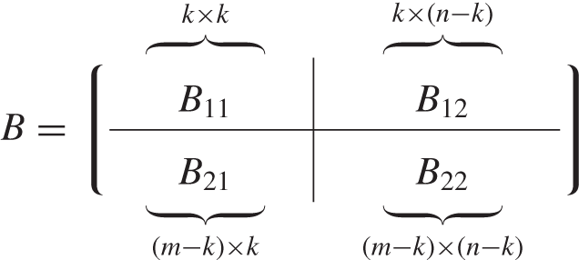
It follows that

$$\Vert A-X{\Vert }_F^2=\Vert B_{11}-{\mathrm{\Omega }}_k{\Vert }_F^2+\Vert B_{12}{\Vert }_F^2+\Vert B_{21}{\Vert }_F^2+\Vert B_{22}{\Vert }_F^2$$

We claim that $B_{12}=O$. If not, then define

$$Y=Q\left[\begin{array}{cc}{B}_{11}& B_{12}\\ O& O\end{array}\right]P^T$$

The matrix Y is in ? and

$$\Vert A-Y{\Vert }_F^2={\Vert B_{21}\Vert }_F^2+{\Vert B_{22}\Vert }_F^2<\Vert A-X{\Vert }_F^2$$

But this contradicts the definition of X. Therefore, $B_{12}=O$. In a similar manner, it can be shown that $B_{21}$ must equal O. If we set

$$Z=Q\left[\begin{array}{cc}{B}_{11}& O\\ O& O\end{array}\right]P^T$$

then $Z\in \mathcal{M}$ and

$$\Vert A-Z{\Vert }_F^2={\Vert B_{22}\Vert }_F^2\le {\Vert B_{11}-{\mathrm{\Omega }}_k\Vert }_F^2+{\Vert B_{22}\Vert }_F^2\Vert A-X{\Vert }_F^2$$

It follows from the definition of X that $B_{11}$ must equal ${\mathrm{\Omega }}_K$. If $B_{22}$ has singular value decomposition $U_1\mathrm{\Lambda }{V}_1^T$, then

$$\Vert A-X{\Vert }_F={\Vert B_{22}\Vert }_F=\Vert \mathrm{\Lambda }{\Vert }_F$$

Let

$$\begin{array}{ccc}{U}_2=\left[\begin{array}{cc}{I}_k& O\\ O& U_1\end{array}\right]& \text{and}& V_2=\left[\begin{array}{cc}{I}_k& O\\ O& V_1\end{array}\right]\end{array}$$

Now,

$$\begin{array}{cc}\hfill U_2^T{Q}^{T}AP{V}_2& =\left[\begin{array}{cc}{\mathrm{\Omega }}_k& O\\ O& \mathrm{\Lambda }\end{array}\right]\hfill \\ \hfill A& =\left(Q{U}_2\right)\left[\begin{array}{cc}{\mathrm{\Omega }}_k& O\\ O& \mathrm{\Lambda }\end{array}\right](P{V}_2{)}^T\hfill \end{array}$$

and hence it follows that the diagonal elements of Λ are singular values of A. Thus,

$$\Vert A-X{\Vert }_F=\Vert \mathrm{\Lambda }{\Vert }_F\ge ({\sigma }_{k+1}^2+\dots +{\sigma }_n^2{)}^{1/2}$$

It then follows from (8) that

$$\Vert A-X{\Vert }_F=({\sigma }_{k+1}^2+\dots +{\sigma }_n^2{)}^{1/2}=\Vert A-A^{\prime }{\Vert }_F$$

∎

If A has singular value decomposition $U\mathrm{\Sigma }{V}^T$, then we can think of A as the product of $U\mathrm{\Sigma }$ times $V^T$. If we partition $U\mathrm{\Sigma }$ into columns and $V^T$ into rows, then

$$U\mathrm{\Sigma }=\left({\sigma }_1{\mathbf{u}}_1,{\sigma }_2{\mathbf{u}}_2,\dots ,\sigma {\mathbf{u}}_n\right)$$

and we can represent A by an outer product expansion

$$A={\sigma }_1{\mathbf{u}}_1{\mathbf{v}}_1^T+{\sigma }_2{\mathbf{u}}_2{\mathbf{v}}_2^T+\dots +{\sigma }_n{\mathbf{u}}_n{\mathbf{v}}_n^T$$ (9)

If A is of rank n, then

$$\begin{array}{cc}\hfill A^{\prime }& =U\left[\begin{array}{ccccc}{\sigma }_1& & & & \\ & {\sigma }_2& & & \\ & & \ddots & & \\ & & & {\sigma }_{n-1}& \\ & & & & 0\end{array}\right]V^T\hfill \\ \hfill & ={\sigma }_1{\mathbf{u}}_1{\mathbf{v}}_1^T+{\sigma }_2{\mathbf{u}}_2{\mathbf{v}}_2^T+\dots +{\sigma }_{n-1}{\mathbf{u}}_{n-1}{\mathbf{v}}_{n-1}^T\hfill \end{array}$$

will be the matrix of rank $n-1$ that is closest to A with respect to the Frobenius norm. Similarly,

$$A^{″}={\sigma }_1{\mathbf{u}}_1{\mathbf{v}}_1^T+{\sigma }_2{\mathbf{u}}_2{\mathbf{v}}_2^T\dots +{\sigma }_{n-2}{\mathbf{u}}_{n-2}{\mathbf{v}}_{n-2}^T$$

will be the nearest matrix of rank $n-2$, and so on. In particular, if A is a nonsingular $n\times n$ matrix, then $A^{\prime }$ is singular and $\Vert A-A^{\prime }{\Vert }_F={\sigma }_n$. Thus, ${\sigma }_n$ may be taken as a measure of how close a square matrix is to being singular.

The reader should be careful not to use the value of det$\left(A\right)$ as a measure of how close A is to being singular. If, for example, A is the $100\times 100$ diagonal matrix whose diagonal entries are all $\frac{{\displaystyle 1}}{{\displaystyle 2}}$, then $\text{det}\left(A\right)=2^{-100}$; however, ${\sigma }_{100}=\frac{{\displaystyle 1}}{{\displaystyle 2}}$. By contrast, the matrix in the next example is very close to being singular even though its determinant is 1 and all its eigenvalues are equal to 1.

Example 3

Let A be an $n\times n$ upper triangular matrix whose diagonal elements are all 1 and whose entries above the main diagonal are all −1:

$$A=\left[\begin{array}{cccccc}1& \hfill -1& \hfill -1& \dots & \hfill -1& \hfill -1\\ 0& \hfill 1& \hfill -1& \dots & \hfill -1& \hfill -1\\ 0& \hfill 0& \hfill 1& \dots & \hfill -1& \hfill -1\\ ⋮& \hfill & & \dots & & \\ 0& \hfill 0& \hfill 0& \dots & \hfill 1& \hfill -1\\ 0& \hfill 0& \hfill 0& \dots & \hfill 0& \hfill 1\end{array}\right]$$

Notice that det$\text{det}\left(A\right)=\text{det}\left(A^{-1}\right)=1$ and all the eigenvalues of A are 1. However, if n is large, then A is close to being singular. To see this, let

$$B=\left[\begin{array}{cccccc}\hfill 1& \hfill -1& \hfill -1& \dots & \hfill -1& \hfill -1\\ \hfill 0& \hfill 1& \hfill -1& \dots & \hfill -1& \hfill -1\\ \hfill 0& \hfill 0& \hfill 1& \dots & \hfill -1& \hfill -1\\ \hfill ⋮& & & \dots & \hfill & \\ \hfill 0& \hfill 0& \hfill 0& \dots & \hfill 1& \hfill -1\\ \hfill \frac{{\displaystyle -1}}{{\displaystyle 2^{n-2}}}& \hfill 0& \hfill 0& \dots & \hfill 0& \hfill 1\end{array}\right]$$

The matrix B must be singular, since the system $B\mathbf{x}=\mathbf{0}$ has a nontrivial solution $\mathbf{x}=(2^{n-2},2^{n-3},\dots ,2^0,1{)}^T$. Since the matrices A and B differ only in the $(n,1)$ position, we have

$$\Vert A-B{\Vert }_F=\frac{{\displaystyle 1}}{{\displaystyle 2^{n-2}}}$$

It follows from Theorem 6.5.3 that

$${\sigma }_n=\underset{X\sin \text{gular}}{\text{min}}\Vert A-X{\Vert }_F\le \Vert A-B{\Vert }_F=\frac{{\displaystyle 1}}{{\displaystyle 2^{n-2}}}$$

Thus, if $n=100$, then ${\sigma }_n\le 1/2^{98}$ and, consequently, A is very close to singular.

∎

Example 4

Suppose that A is a $5\times 5$ matrix with singular values

$${\sigma }_1=4,{\sigma }_2=1,{\sigma }_3={10}^{-12},{\sigma }_4=3.1\times {10}^{-14},{\sigma }_5=2.6\times {10}^{-15}$$

and suppose that the machine epsilon is $5\times {10}^{-15}$. To determine the numerical rank, we compare the singular values to

$${\sigma }_1\text{max}(m,n)\in =\mathrm{4.5.5}\times {10}^{-15}={10}^{-13}$$

Since three of the singular values are greater than ${10}^{-13}$, the matrix has numerical rank 3.

∎