
7 Experimentation in action: Moving from prototype to MVP
- Techniques for hyperparameter tuning and the benefits of automated approaches
- Execution options for improving the performance of hyperparameter optimization
In the preceding chapter, we explored the scenario of testing and evaluating potential solutions to a business problem focused on forecasting passengers at airports. We ended up arriving at a decision on the model to use for the implementation (Holt-Winters exponential smoothing) but performed only a modicum of model tuning during the rapid prototyping phases.
Moving from experimental prototyping to MVP development is challenging. It requires a complete cognitive shift that is at odds with the work done up to this point. We’re no longer thinking of how to solve a problem and get a good result. Instead, we’re thinking of how to build a solution that is good enough to solve the problem in a way that is robust enough so that it’s not breaking constantly. We need to shift focus to monitoring, automated tuning, scalability, and cost. We’re moving from scientific-focused work to the realm of engineering.
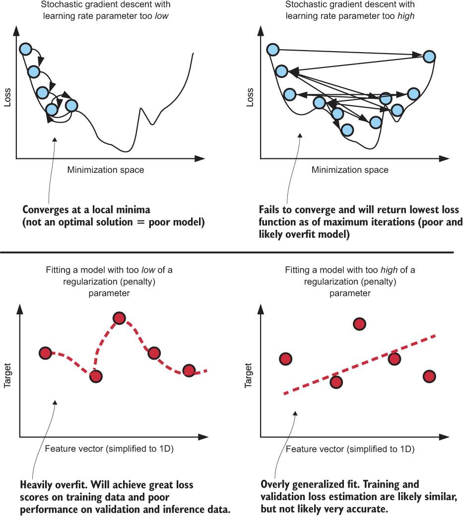
The first priority when moving from prototype to MVP is ensuring that a solution is tuned correctly. See the following sidebar for additional details on why it’s so critical to tune models and how these seemingly optional settings in modeling APIs are actually important to test.
7.1 Tuning: Automating the annoying stuff
Throughout the last two chapters, we’ve been focusing on a peanut forecasting problem. At the end of chapter 6, we had a somewhat passable prototype, validated on a single airport. The process used to adjust and tune the predictive performance of the model was manual and not particularly scientific, and left a large margin between what is possible for the model’s predictive ability and what we had manually tuned.
In this scenario, the difference between OK and very good predictions could be a large margin of product that we want to stage at airports. Being off in our forecasts, after all, could translate to many millions of dollars. Spending time manually tuning by just trying a bunch of hyperparameters simply won’t scale for predictive accuracy or for timeliness of delivery.
If we want to come up with a better approach than tribal-knowledge guessing for tuning the model, we need to look at our options. Figure 7.1 shows various approaches that DS teams use to tune models, progressing in order from simple (less powerful and maintainable) to complex (custom framework).
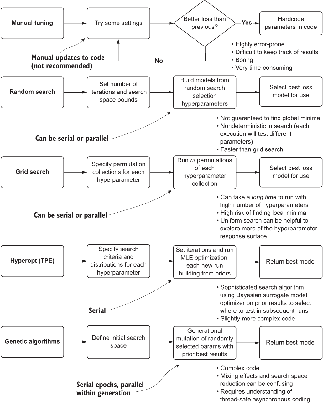
Figure 7.1 Comparison of hyperparameter tuning approaches
The top section, manual tuning, is typically how prototypes are built. Manually testing values of hyperparameters, when doing rapid testing, is an understandable approach. The goal of the prototype, as mentioned in chapter 6, is getting an approximation of the tunability of a solution. At the stage of moving toward a production-capable solution, however, more maintainable and powerful solutions need to be considered.
7.1.1 Tuning options
We know that we need to tune the model. In chapter 6, we saw clearly what happens if we don’t do that: generating a forecast so laughably poor that pulling numbers from a hat would be more accurate. However, multiple options could be pursued to arrive at the most optimal set of hyperparameters.
Manual tuning (educated guessing)
We will see later, when applying Hyperopt to our forecasting problem, just how difficult it will be to arrive at the optimal hyperparameters for each model that needs to be built for this project. Not only are the optimized values unintuitive to guess at, but each forecasting model’s optimal hyperparameter set is different from that of other models.
Getting even remotely close to optimal parameters with a manual testing methodology is unlikely. The process is inefficient, frustrating, and an incredible waste of time to attempt, as shown in figure 7.2.
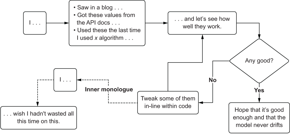
Figure 7.2 The acute pain of manual hyperparameter tuning
Tip Don’t try manual tuning unless you’re working with an algorithm that has a very small number of hyperparameters (one or two, preferably Boolean or categorical).
The primary issue with this method is in tracking what has been tested. Even if a system was in place to record and ensure that the same values haven’t been tried before, the sheer amount of work required to maintain that catalog is overwhelming, prone to errors, and pointless in the extreme.
Project work, after the rapid prototyping phase, should always abandon this approach to tuning as soon as is practicable. You have so many better things to do with your time, believe me.
A cornerstone of ML techniques, the brute-force-search approach of grid-based testing of hyperparameters has been around for quite some time. To perform a grid search, the DS will select a set collection of values to test for each hyperparameter. The grid search API will then assemble collections of hyperparameters to test by creating permutations of each value from each group that has been specified. Figure 7.3 illustrates how this works, as well as why it might not be something that you would entertain for models with a lot of hyperparameters.
As you can see, with high hyperparameter counts, the sheer number of permutations that need to be tested can quickly become overwhelming. The trade-off, clearly, is between the time required to run all of the permutations and the search capability of the optimization. If you want to explore more of the hyperparameter response surface, you’re going to have to run more iterations. There’s really no free lunch here.
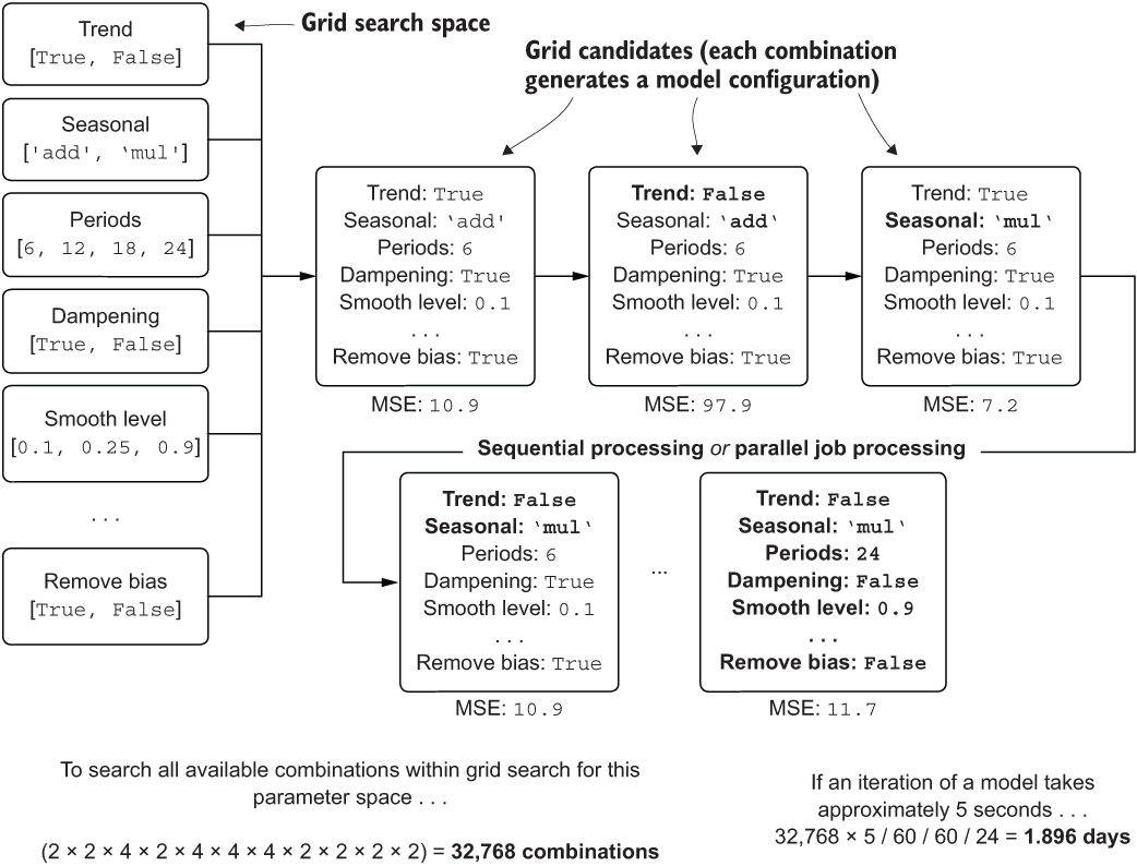
Figure 7.3 Brute-force grid search approach to tuning
With all of the grid search’s limitations that hamper its ability to arrive at an optimized set of hyperparameters, using it can be prohibitively expensive in terms of both time and money. Were we interested in thoroughly testing all continuously distributed hyperparameters in a forecasting model, the amount of time to get an answer, when running on a single CPU, would be measured in weeks rather than minutes.
An alternative to grid search, to attempt to simultaneously test the influencing effects of different hyperparameters at the same time (rather than relying on explicit permutations to determine the optimal values), is using random sampling of each of the hyperparameter groups. Figure 7.4 illustrates random search; compare it to figure 7.3 to see the differences in the approaches.

Figure 7.4 Random search process for hyperparameter optimization
As you can see, the selection of candidates to test is random and is controlled not through the mechanism of permutations of all possible values, but rather through a maximum number of iterations to test. This is a bit of a double-edged sword: although the execution time is dramatically reduced, the search through the hyperparameter space is limited.
Model-based optimization: Tree-structured Parzen estimators (Hyperopt)
We face a complex search for hyperparameters in our time-series forecasting model—11 total hyperparameters, 3 continuously distributed and 1 ordinal—confounding the ability to effectively search the space. The preceding approaches are either too time-consuming (manual, grid search), expensive (grid search), or difficult to achieve adequate fit characteristics for validation against holdout data (all of them).
The same team that brought the paper arguing that random search is a superior methodology to grid search also arrived at a process for selecting an optimized hyperparameter response surface: using Bayesian techniques in a model-based optimization relying on either Gaussian processes or tree of Parzen estimators (TPEs). The results of their research are provided in the open source software package Hyperopt. Figure 7.5 shows at a high level how Hyperopt works.
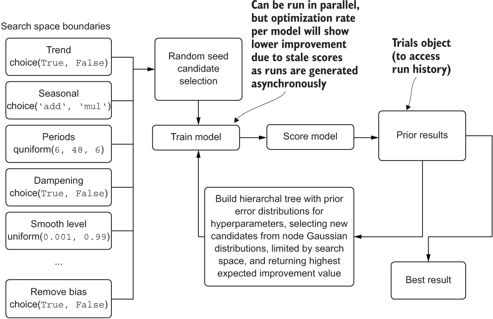
Figure 7.5 A high-level diagram of how Hyperopt’s tree-structured Parzen estimator algorithm works
This system is nearly guaranteed to outperform even the most experienced DS working through any of the earlier mentioned classical tuning approaches. Not only is it remarkably capable of exploring complex hyperparameter spaces, but it can do so in far fewer iterations than other methodologies. For further reading on this topic, I recommend perusing the original 2011 whitepaper, “Algorithms for Hyper-Parameter Optimization” by James Bergstra et al. (http://mng.bz/W76w) and reading the API documentation for the package for further evidence of its effectiveness (http://hyperopt.github.io/hyperopt/).
More advanced (and complex) techniques
Anything more advanced than Hyperopt’s TPE and similar automated tuning packages typically means doing one of two things: paying a company that offers an automated-ML (autoML) solution or building your own. In the realm of building a custom tuner solution, you might look into a mixture of genetic algorithms with Bayesian prior search optimization to create search candidates within the n-dimensional hyperparameter space that have the highest likelihood of giving a good result, leveraging the selective optimization that genetic algorithms are known for.
Speaking from the perspective of someone who has built one of these autoML solutions (https://github.com/databrickslabs/automl-toolkit), I cannot recommend going down this path unless you’re building out a custom framework for hundreds (or more) different projects and have a distinct need for a high-performance and lower-cost optimization tool specifically customized to solve the sorts of problems that your company is facing.
AutoML is definitely not a palatable option for most experienced DS teams, however. The very nature of these solutions, being largely autonomous apart from a configuration-driven interface, forces you to relinquish control and visibility into the decision logic contained within the software. You lose the ability to discover the reasoning behind why some features are culled and others are created, why a particular model was selected, and what internal validations may have been performed on your feature vector to achieve the purported best results.
Setting aside that these solutions are black boxes, it’s important to recognize the target audience for these applications. These full-featured pipeline-generation toolkits are not designed or intended for use by seasoned ML developers in the first place. They’re built for the unfortunately named citizen data scientist—the SMEs who know their business needs intimately but don’t have the experience or knowledge to handcraft an ML solution by themselves.
Building a framework to automate some of the more (arguably) boring and rudimentary modeling needs that your company faces may seem exciting. It certainly can be. These frameworks aren’t exactly simple to build, though. If you’re going down the path of building something custom, like an autoML framework, make sure that you have the bandwidth to do so, that the business understands and approves of this massive project, and that you can justify your return on a substantial investment of time and resources. During the middle of a project is not the time to tack on months of cool work.
7.1.2 Hyperopt primer
Going back to our project work with forecasting, we can confidently assert that the best approach for tuning the models for each airport is going to be through using Hyperopt and its TPE approach.
NOTE Hyperopt is a package that is external to the build of Anaconda we’ve been using. To use it, you must perform a pip or conda install of the package in your environment.
Before we get into the code that we’ll be using, let’s look at how this API works from a simplified implementation perspective. To begin, the first aspect of Hyperopt is in the definition of an objective function (listing 7.1 shows a simplified implementation of a function for finding a minimization). This objective function is, typically, a model that is fit on training data, validated on testing data, scored, and returns the error metric associated with the predicted data as compared to the validation data.
Listing 7.1 Hyperopt fundamentals: The objective function
import numpy as np
def objective_function(x):                   ❶
  func = np.poly1d([1, -3, -88, 112, -5])    ❷
  return func(x) * 0.01                      ❸
❶ Defines the objective function to minimize
❷ A one-dimensional fourth-order polynomial equation that we want to solve for
❸ Loss estimation for the minimization optimization
After we have declared an objective function, the next phase in using Hyperopt is to define a space to search over. For this example, we’re interested in only a single value to optimize for, in order to solve the minimization of the polynomial function in listing 7.1. In the next listing, we define the search space for this one x variable for the function, instantiating the Trials object (for recording the history of the optimization), and running the optimization with the minimization function from the Hyperopt API.
Listing 7.2 Hyperopt optimization for a simple polynomial
optimization_space = hp.uniform('x', -12, 12)     ❶
trials = Trials()                                 ❷
trial_estimator = fmin(fn=objective_function,     ❸
                       space=optimization_space,  ❹
                       algo=tpe.suggest,          ❺
                       trials=trials,             ❻
                       max_evals=1000             ❼
)
❶ Defines the search space—in this case, a uniform sampling between -12 and 12 for the seed and bounded Gaussian random selection for the TPE algorithm after the initial seed priors return
❷ Instantiates the Trials object to record the optimization history
❸ The objective function as defined in listing 7.1, passed in to the fmin optimization function of Hyperopt
❹ The space to search, defined above (-12 to 12, uniformly)
❺ The optimization algorithm to use—in this case, tree-structured Parzen estimator
❻ Passes the Trials object into the optimization function to record the history of the run
❼ The number of optimization runs to conduct. Since hpopt is iterations-bound, we can control the runtime of the optimization in this manner.
Once we execute this code, we will receive a progress bar (in Jupyter-based notebooks) that will return the best loss that has been discovered throughout the history of the run as it optimizes. At the conclusion of the run, we will get as a return value from trial_estimator the optimal setting for x to minimize the value returned from the polynomial defined in the function objective_function. The following listing shows how this process works for this simple example.
Listing 7.3 Hyperopt performance in minimizing a simple polynomial function
rng = np.arange(-11.0, 12.0, 0.01)                                    ❶
values = [objective_function(x) for x in rng]                         ❷
with plt.style.context(style='seaborn'):
  fig, ax = plt.subplots(1, 1, figsize=(5.5, 4))
  ax.plot(rng, values)                                                ❸
  ax.set_title('Objective function')
  ax.scatter(x=trial_estimator[‘x’], y=trials.average_best_error(), marker='o', s=100)                                               ❹
  bbox_text = 'Hyperopt calculated minimum value
x: {}'.format(trial_estimator['x'])
  arrow = dict(facecolor='darkblue', shrink=0.01, connectionstyle='angle3,angleA=90,angleB=45')
  bbox_conf = dict(boxstyle='round,pad=0.5', fc='ivory', ec='grey', lw=0.8)
  conf = dict(xycoords='data', textcoords='axes fraction', arrowprops=arrow, bbox=bbox_conf, ha='left', va='center', fontsize=12)
  ax.annotate(bbox_text, xy=(trial_estimator['x'], trials.average_best_error()), xytest=(0.3, 0.8), **conf)         ❺
  fig.tight_layout()
  plt.savefig('objective_func.svg', format='svg')
❶ Generates a range of x values for plotting the function defined in listing 7.1
❷ Retrieves the corresponding y values for each of the x values from the rng collection
❸ Plots the function across the x space of rng
❹ Plots the optimized minima that Hyperopt finds based on our search space
❺ Adds an annotation to the graph to indicate the minimized value
Running this script results in the plot in figure 7.6.
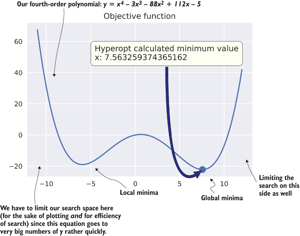
Figure 7.6 Using Hyperopt to solve for the minimal value of a simple polynomial
Linear models frequently have “dips” and “valleys” between parameters and their loss metrics. We use the terms local minima and local maxima to describe them. If the parameter search space isn’t explored sufficiently, a model’s tuning could reside in a local, instead of the global, minima or maxima.
7.1.3 Using Hyperopt to tune a complex forecasting problem
Now that you understand the concepts behind this automated model-tuning package, we can apply it to our complex forecasting modeling problem. As we discussed earlier in this chapter, tuning this model is going to be complex if we don’t have some assistance. Not only are there 11 hyperparameters to explore, but the success that we had in chapter 6 at manually tuning was not particularly impressive.
We need something to help us. Let’s let Thomas Bayes lend a hand (or, rather, Pierre-Simon Laplace). Listing 7.4 shows our optimization function for the Holt-Winters exponential smoothing (HWES) model for passengers at airports.
Listing 7.4 Minimization function for Holt-Winters exponential smoothing
def hwes_minimization_function(selected_hp_values, train, test, loss_metric):❶
    model = ExponentialSmoothing(train,                                      ❷
                   trend=selected_hp_values['model']['trend'],
                   seasonal=selected_hp_values['model']['seasonal'],
                   seasonal_periods=selected_hp_values['model'][                'seasonal_periods'],
                   damped=selected_hp_values['model']['damped']
                   )
    model_fit =                                                             ❸
    model.fit(smoothing_level=selected_hp_values['fit']['smoothing_level'],
                smoothing_seasonal=selected_hp_values['fit'][             'smoothing_seasonal'],
                damping_slope=selected_hp_values['fit']['damping_slope'],
                use_brute=selected_hp_values['fit']['use_brute'],
                use_boxcox=selected_hp_values['fit']['use_boxcox'],
                use_basinhopping=selected_hp_values['fit'][             'use_basinhopping'],
                remove_bias=selected_hp_values['fit']['remove_bias']
                )
    forecast = model_fit.predict(train.index[-1], test.index[-1])            ❹
    param_count = extract_param_count_hwes(selected_hp_values)               ❺
    adjusted_forecast = forecast[1:]                                         ❻
    errors = calculate_errors(test, adjusted_forecast, param_count)          ❼
    return {'loss': errors[loss_metric], 'status': STATUS_OK}                ❽
❶ selected_hp_values is a multilevel dictionary. Since we have two separate sections of hyperparameters to apply and some of the parameter names are similar, we separate them between “model” and “fit” to reduce confusion.
❷ Instantiates the ExponentialSmoothing class as an object, configured with the values that Hyperopt will be selecting for each model iteration to test
❸ The fit method has its own set of hyperparameters that Hyperopt will be selecting for the pool of models it will generate and test.
❹ Generates the forecast for this run of the model to perform validation and scoring against. We are forecasting from the point of the end of the training set to the last value of the test set’s index.
❺ A utility function to get the number of parameters (viewable in the book’s GitHub repository)
❻ Removes the first entry of the forecast since it overlaps with the training set’s last index entry
❼ Calculates all of the error metrics—Akaike information criterion (AIC) and Bayesian information criterion (BIC), newly added metrics, requires the hyperparameter count
❽ The only return from the minimization function for Hyperopt is a dictionary containing the metric under test for optimization and a status report message from within the Hyperopt API. The Trials() object will persist all of the data about the runs and a tuned best model.
As you may recall from chapter 6, when creating the prototype for this algorithm, we hardcoded several of these values (smoothing_level, smoothing_seasonal, use_brute, use_boxcox, use_basin_hopping, and remove_bias) to make the prototyping tuning a bit easier. In listing 7.4, we’re setting all of these values as tunable hyperparameters for Hyperopt. Even with such a large search space, the algorithm will allow us to explore the influence of all of them over the predictive capabilities of the holdout space. If we were using something permutations-based (or, worse, human-short-term-memory-based) such as a grid search, we likely wouldn’t want to include all of these for the sole reason of factorially increasing runtime.
Now that we have our model-scoring implementation done, we can move on to the next critical phase of efficiently tuning these models,: defining the search space for the hyperparameters.
Listing 7.5 Hyperopt exploration space configuration
hpopt_space = {
    'model': {                                                             ❶
          'trend': hp.choice('trend', ['add', 'mul']),                     ❷
          'seasonal': hp.choice('seasonal', ['add', 'mul']),
          'seasonal_periods': hp.quniform('seasonal_periods', 12, 120, 12),❸
          'damped': hp.choice('damped', [True, False])
    },
    'fit': {
          'smoothing_level': hp.uniform('smoothing_level', 0.01, 0.99),    ❹
          'smoothing_seasonal': hp.uniform('smoothing_seasonal', 0.01, 0.99),
          'damping_slope': hp.uniform('damping_slope', 0.01, 0.99),
          'use_brute': hp.choice('use_brute', [True, False]),
          'use_boxcox': hp.choice('use_boxcox', [True, False]),
          'use_basinhopping': hp.choice('use_basinhopping', [True, False]),
          'remove_bias': hp.choice('remove_bias', [True, False])
    }
}
❶ For readability’s sake, we’re splitting the configuration between the class-level hyperparameters (model) and the method-level hyperparameters (fit) since some of the names for the two are similar.
❷ hp.choice is used for Boolean and multivariate selection (choose one element from a list of possible values).
❸ hp.quniform chooses a random value uniformly in a quantized space (in this example, we’re choosing a multiple of 12, between 12 and 120).
❹ hp.uniform selects randomly through the continuous space (here, between 0.01 and 0.99).
The settings in this code are the total sum of hyperparameters available for the ExponentialSmoothing() class and the fit() method as of statsmodels version 0.11.1. Some of these hyperparameters may not influence the predictive power of our model. If we had been evaluating this through grid search, we would likely have omitted them from our evaluation. With Hyperopt, because of the manner in which its algorithm provides greater weight to influential parameters, leaving them in for evaluation doesn’t dramatically increase the total runtime.
The next step for automating away the daunting task of tuning this temporal model is to build a function to execute the optimization, collect the data from the tuning run, and generate plots that we can use to further optimize the search space as defined in listing 7.5 on subsequent fine-tuning runs. Listing 7.6 shows our final execution function.
NOTE Please refer to the companion repository to this book at https://github.com/BenWilson2/ML-Engineering to see the full code for all of the functions called in listing 7.6. A more thorough discussion is included there in a downloadable and executable notebook.
Listing 7.6 Hyperopt tuning execution
def run_tuning(train, test, **params):                                   ❶
    param_count = extract_param_count_hwes(params['tuning_space'])       ❷
    output = {}
    trial_run = Trials()                                                 ❸
    tuning = fmin(partial(params['minimization_function'],               ❹
                          train=train,
                          test=test,
                          loss_metric=params['loss_metric']
                         ),
                  params['tuning_space'],                                ❺
                  algo=params['hpopt_algo'],                             ❻
                  max_evals=params['iterations'],                        ❼
                  trials=trial_run
                 )
    best_run = space_eval(params['tuning_space'], tuning)                ❽
    generated_model = params['forecast_algo'](train, test, best_run)     ❾
    extracted_trials = extract_hyperopt_trials(trial_run, params['tuning_space'], params['loss_metric'])                      ❿
    output['best_hp_params'] = best_run
    output['best_model'] = generated_model['model']
    output['hyperopt_trials_data'] = extracted_trials
    output['hyperopt_trials_visualization'] =  generate_hyperopt_report(extracted_trials, params['loss_metric'], params['hyperopt_title'], params['hyperopt_image_name'])            ⓫
    output['forecast_data'] = generated_model['forecast']
    output['series_prediction'] = build_future_forecast(
                                                generated_model['model'],
                                                params['airport_name'],
                                                params['future_forecast_                                                  periods'],
                                                params['train_split_cutoff_                                                  months'],
                                                params['target_name']
                                                       )                 ⓬
    output['plot_data'] = plot_predictions(test,
                                           generated_model['forecast'],
                                           param_count,
                                           params['name'],
                                           params['target_name'],
                                           params['image_name'])         ⓭
    return output
❶ Because of the volume of configurations used to execute the tuning run and collect all the visualizations and data from the optimization, we’ll use named dictionary-based argument passing (**kwargs).
❷ To calculate AIC and BIC, we need the total number of hyperparameters being optimized. Instead of forcing the user of this function to count them, we can extract them from the passed-in Hyperopt configuration element tuning_space.
❸ The Trials() object records each of the, well, trials of different hyperparameter experiments and allows us to see how the optimization converged.
❹ fmin() is the main method for initiating a Hyperopt run. We’re using a partial function as a wrapper around the per-model static attributes so that the sole differences between each Hyperopt iteration is in the variable hyperparameters, keeping the other attributes the same.
❺ The tuning space defined in listing 7.5
❻ The optimization algorithm for Hyperopt (random, TPE, or adaptive TPE), which can be automated or manually controlled
❼ The number of models to test and search through to find an optimal configuration
❽ Extracts the best model from the Trials() object
❾ Rebuilds the best model to record and store
❿ Pulls the tuning information out of the Trials() object for plotting
⓬ Builds the future forecast for as many points as specified in the future_forecast_periods configuration value
⓭ Plots the forecast over the holdout validation period to show test vs. forecast (updated version from chapter 6 visualization)
note To read more about how partial functions and Hyperopt work, see the Python documentation at https://docs.python.org/3/library/functools.html#functools.partial and the Hyperopt doc and source code at https://github.com/hyperopt/hyperopt.github.io.
Note Listing 7.6’s custom plot code is available in the companion repository for this book; see the Chapter7 notebook at https://github.com/BenWilson2/ML-Engineering.
Executing the call to plot_predictions() from listing 7.6 is shown in figure 7.7. Calling generate_hyperopt_report() from listing 7.6 results in the plot shown in figure 7.8.
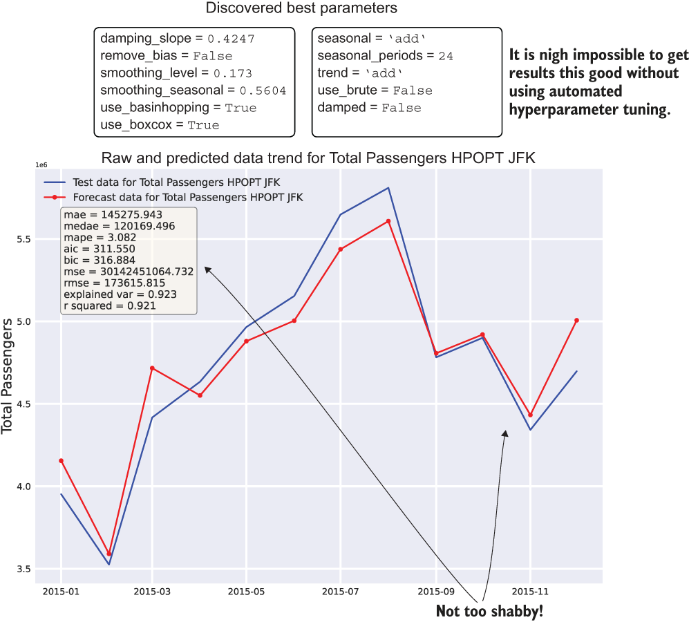
Figure 7.7 Prediction backtesting on the most recent data from the total time series (x-axis zoomed for legibility)
By using Hyperopt to arrive at the best predictions on our holdout data, we’ve optimized the hyperparameters to a degree that we can be confident of having a good projection of the future state (provided that no unexpected and unknowable latent factors affect it). Thus, we’ve addressed several key challenging elements in the optimization phase of ML work by using automated tuning:
- Accuracy—The forecast is as optimal as it can be (for each model, provided that we select a reasonable search space and run through enough iterations).
- Timeliness in training—With this level of automation, we get well-tuned models in minutes instead of days (or weeks).
- Maintainability—Automating tuning keeps us from having to manually retrain models as the baseline shifts over time.
- Timeliness in development—Since our code is pseudo-modular (using modularized functions within a notebook), the code is reusable, extensible, and capable of being utilized through a control loop to build all the models for each airport with ease.
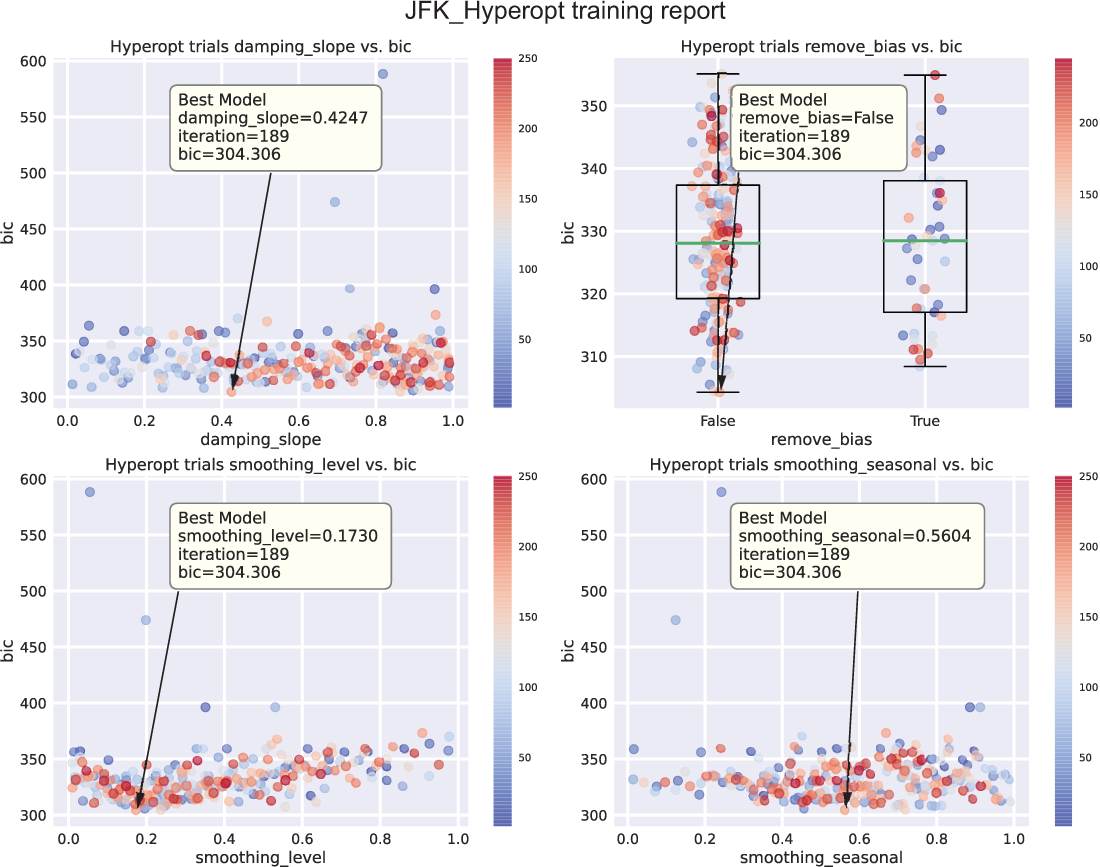
Figure 7.8 Sampled results of hyperparameters for the Hyperopt trials run
NOTE The extracted code samples that we’ve just gone through with Hyperopt are part of a much larger end-to-end example hosted within the book’s repository in the Notebooks section for chapter 7. In this example, you can see the automated tuning and optimization for all airports within this dataset and all utility functions that are built to support this effective tuning of models.
7.2 Choosing the right tech for the platform and the team
The forecasting scenario we’ve been walking through, when executed in a virtual machine (VM) container and running automated tuning optimization and forecasting for a single airport, worked quite well. We got fairly good results for each airport. By using Hyperopt, we also managed to eliminate the unmaintainable burden of manually tuning each model. While impressive, it doesn’t change the fact that we’re not looking to forecast passengers at just a single airport. We need to create forecasts for thousands of airports.
Figure 7.9 shows what we’ve built, in terms of wall-clock time, in our efforts thus far. The synchronous nature of each airport’s models (in a forloop) and Hyperopt’s Bayesian optimizer (also a serial loop) means that we’re waiting for models to be built one by one, each next step waiting on the previous to be completed, as we discussed in section 7.1.2.
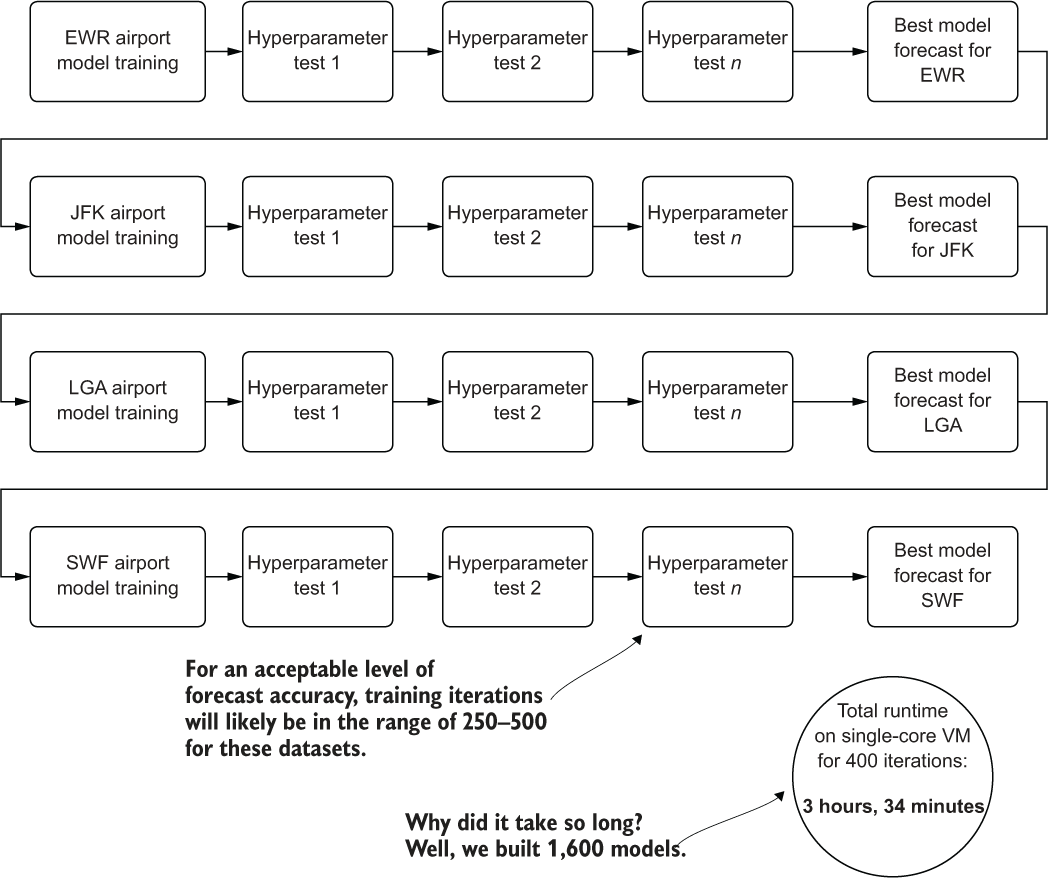
Figure 7.9 Serial tuning in single-threaded execution
This problem of ML at scale, as shown in this diagram, is a stumbling block for many teams, mostly because of complexity, time, and cost (and is one the primary reasons why projects of this scale are frequently cancelled). Solutions exist for these scalability issues for ML project work; each involves stepping away from the realm of serial execution and moving into the world of distributed, asynchronous, or a mixture of both of these paradigms of computing.
The standard structured code approach for most Python ML tasks is to execute in a serial fashion. Whether it be a list comprehension, a lambda, or a for (while) loop, ML is steeped in sequential execution. This approach can be a benefit, as it reduces memory pressure for many algorithms that have a high memory requirement, particularly those that use recursion, which are many. But this approach can also be a handicap, as it takes much longer to execute, since each subsequent task is waiting for the previous to complete.
We will discuss concurrency in ML briefly in section 7.4 and in more depth in later chapters (both safe and unsafe ways of doing it). For now, with the issue of scalability with respect to wall-clock time for our project, we need to look into a distributed approach to this problem in order to explore our search spaces faster for each airport. It is at this point that we stray from the world of our single-threaded VM approach and move into the distributed computing world of Apache Spark.
7.2.1 Why Spark?
Why use Spark? In a word: speed.
For the problem that we’re dealing with here, forecasting each month the passenger expectations at each major airport in the United States, we’re not bound by SLAs that are measured in minutes or hours, but we still need to think about the amount of time it takes to run our forecasting. There are multiple reasons for this, chiefly
- Time—If we’re building this job as a monolithic modeling event, any failures in an extremely long-running job will require a restart (imagine the job failing after it was 99% complete, running for 11 days straight).
- Stability—We want to be very careful about object references within our job and ensure that we don’t create a memory leak that could cause the job to fail.
- Risk—Keeping machines dedicated to extremely long-running jobs (even in cloud providers) risks platform issues that could bring down the job.
- Cost—Regardless of where your virtual machines are running, someone is paying the bill for them.
When we focus on tackling these high-risk factors, distributed computing offers a compelling alternative to serial looped execution, not only because of cost, but mostly because of the speed of execution. Were any issues to arise in the job, unforeseen issues with the data, or problems with the underlying hardware that the VMs are running on, these dramatically reduced execution times for our forecasting job will give us flexibility to get the job up and running again with predicted values returning much faster.
But how is Spark going to help us with this problem? We can employ two relatively straightforward paradigms, shown in figure 7.10. We could use more than just these two, but we’re going to start with the straightforward and less complex ones for now; the more advanced approaches are mentioned in section 7.4.
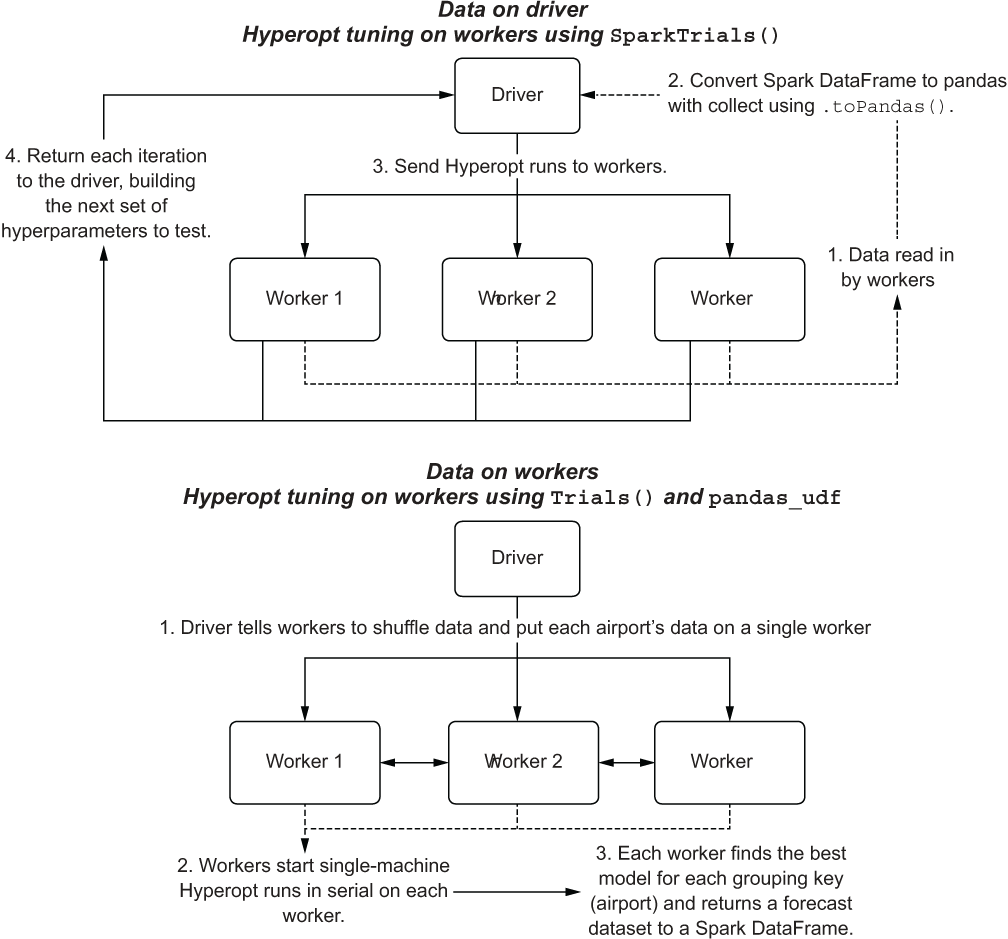
Figure 7.10 Scaling hyperparameter tuning using pandas_udf on Spark
The first approach is to leverage the workers within the cluster to execute parallel evaluation of the hyperparameters. In this paradigm, our time-series dataset will need to be collected (materialized in full) from the workers to the driver. Limitations exist (serialization size of the data is currently limited to 2 GB at the time of this writing), and for many ML use cases on Spark, this approach shouldn’t be used. For time-series problems such as this one, this approach will work just fine.
In the second approach, we leave the data on the workers. We utilize pandas_udf to distribute concurrent training of each airport on each worker by using our standalone Hyperopt Trials() object, just as we did in chapter 6 when running on a single-core VM.
Now that we’ve defined the two paradigms for speeding up hyperparameter tuning from a high-level architectural perspective, let’s look at the process execution (and trade-offs of each) in the next two subsections.
7.2.2 Handling tuning from the driver with SparkTrials
While figure 7.10 shows the physical layout of the operations occurring within a Spark cluster for handling distributed tuning with SparkTrials(), figure 7.11 shows the execution in more detail. Each airport that needs to be modeled is iterated over on the driver, its optimization handled through a distributed implementation wherein each candidate hyperparameter collection is submitted to a different worker.
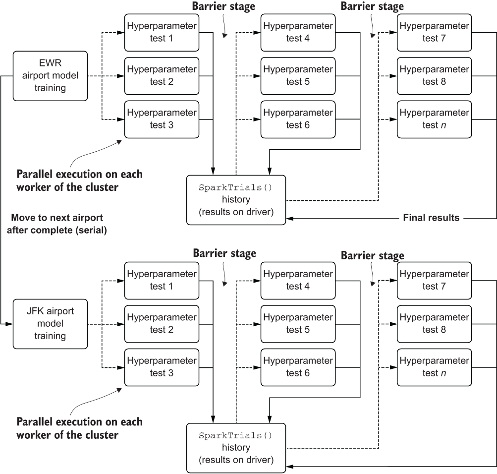
Figure 7.11 Logical architecture of utilizing Spark workers to distribute Hyperopt test iterations for hyperparameter optimization
This approach works remarkably well with a minimal amount of modification to achieve a similar level of hyperparameter space searching as compared to the single-core approach, needing only a small increase to the number of iterations as the level of parallelism is increased.
NOTE Increasing the number of iterations as a factor of the parallelism level is not advisable. In practice, I generally increase the iterations by a simple adjustment of the number of single-core iterations + (parallelism factor / 0.2). This is to give a larger pool of prior values to pull from. With parallel runs executing asynchronously, each boundary epoch that is initiated will not have the benefit of in-flight results that a synchronous execution would.
This is so critical to do because of the nature of the optimizer in Hyperopt. Being a Bayesian estimator, the power of its ability to arrive at an optimized set of parameters to test lies directly in its access to prior data. If too many runs are executing concurrently, the lack of data on their results translates to a higher rate of searching through parameters that have a lower probability to work well. Without the prior results, the optimization becomes much more of a random search, defeating the purpose of using the Bayesian optimizer.
This trade-off is negligible, though, particularly when compared to the rather impressive performance achievable by utilizing n workers to distribute each iteration to. To port our functions over to Spark, only a few changes need to happen for this first paradigm.
NOTE To follow along fully with a referenceable and executable example of distributed hyperparameter optimization with Apache Spark, please see the companion Spark notebook in the book’s repository entitled Chapter8_1, which we will be using throughout the next chapter as well.
The first thing that we’ll need to do is to import the module SparkTrials from Hyperopt. SparkTrials is a tracking object that allows for the cluster’s driver to maintain a history of all the experiments that have been attempted with different hyperparameter configurations executed on the remote workers (as opposed to the standard Trials object that tracks the history of runs conducted on the same VM).
Once we have the import completed, we can read in our data by using a native Spark reader (in this instance, our data has been stored in a Delta table and registered to the Apache Hive Metastore, making it available through the standard database and table name identifiers). Once we have the data loaded onto the workers, we can then collect the series data to the driver, as shown in the following listing.
Listing 7.7 Using Spark to collect data to the driver as a pandas DataFrame
delta_table_nm = 'airport'                                          ❶
delta_database_nm = 'ben_demo'                                      ❷
delta_full_nm = "{}.{}".format(delta_database_nm, delta_table_nm)   ❸
local_data = spark.table(delta_full_nm).toPandas()                  ❹
❶ Defines the name of the Delta table that we’ve written the airport data to
❷ Defines the name of the Hive database that the Delta table is registered to
❸ Interpolates the database name and the table name into standard API signature for data retrieval
❹ Reads in the data with the workers from Delta (there is no ability to directly read in data to the driver from Delta), and then collects the data to the driver node as a pandas DataFrame
WARNING Be careful about collecting data in Spark. With the vast majority of large-scale ML (with a training dataset that could be in the tens or hundreds of gigabytes), a .toPandas() call, or any collect action at all, in Spark will fail. If you have a large collection of data that can be iterated through, simply filter the Spark DataFrame and use an iterator (loop) to collect chunks of the data with a .toPandas() method call to control the amount of data being processed on the driver at a time.
After running the preceding code, we are left with our data residing on the driver, ready for utilizing the distributed nature of the Spark cluster to conduct a far more scalable tuning of the models than what we were dealing with in our Docker container VM from section 7.1. The following listing shows the modifications to listing 7.6 that allow us to run in this manner.
Listing 7.8 Modifying the tuning execution function for running Hyperopt on Spark
def run_tuning(train, test, **params):
    param_count = extract_param_count_hwes(params['tuning_space'])
    output = {}
    trial_run = SparkTrials(parallelism=params['parallelism'], timeout=params['timeout'])                                           ❶
    with mlflow.start_run(run_name='PARENT_RUN_{}'.format(params['airport_name']), nested=True):                                      ❷
      mlflow.set_tag('airport', params['airport_name'])                    ❸
      tuning = fmin(partial(params['minimization_function'],
                            train=train,
                            test=test,
                            loss_metric=params['loss_metric']
                           ),
                    params['tuning_space'],
                    algo=params['hpopt_algo'],
                    max_evals=params['iterations'],
                    trials=trial_run,
                    show_progressbar=False
                   )                                                      ❹
      best_run = space_eval(params['tuning_space'], tuning)
      generated_model = params['forecast_algo'](train, test, best_run)
      extracted_trials = extract_hyperopt_trials(trial_run,
        params['tuning_space'], params['loss_metric'])
      output['best_hp_params'] = best_run
      output['best_model'] = generated_model['model']
      output['hyperopt_trials_data'] = extracted_trials
      output['hyperopt_trials_visualization'] =
        generate_Hyperopt_report(extracted_trials,
                               params['loss_metric'],
                               params['hyperopt_title'],
                               params['hyperopt_image_name'])
      output['forecast_data'] = generated_model['forecast']
      output['series_prediction'] = build_future_forecast(
                                          generated_model['model'],
                                          params['airport_name'],
                                          params['future_forecast_periods'],
                                          params['train_split_cutoff_months'],
                                          params['target_name'])
      output['plot_data'] = plot_predictions(test,
                                             generated_model['forecast'],
                                             param_count,
                                             params['name'],
                                             params['target_name'],
                                             params['image_name'])
      mlflow.log_artifact(params['image_name'])                            ❺
      mlflow.log_artifact(params['hyperopt_image_name'])                    ❻
    return output
❶ Configures Hyperopt to use SparkTrials() instead of Trials(), setting the number of concurrent experiments to run on the workers in the cluster and the global time-out level (since we’re using Futures to submit the tests)
❷ Configures MLflow to log the results of each hyperparameter test within a parent run for each airport
❸ Logs the airport name to MLflow to make it easier to search through the results of the tracking service
❹ The minimization function remains largely unchanged with the exception of adding in MLflow logging of both the hyperparameters and the calculated loss metrics that are being tested for the iteration within the child run.
❺ Logs the generated prediction plots for the best model to the parent MLflow run
❻ Logs the Hyperopt report for the run, written to the parent MLflow run ID
Little modification needed to happen to the code to get it to work within the distributed framework of Spark. As a bonus (which we will discuss in more depth in section 7.3), we can also log information with ease to MLflow, solving one of our key needs for creating a maintainable project: provenance of tests for reference and comparison.
Based on the side-by-side comparison of this methodology to that of the run conducted in our single-core VM, this approach meets the goals of timeliness that we were searching for. We’ve reduced the optimization phase of this forecasting effort from just over 3.5 hours to, on a relatively small four-node cluster, just under 30 minutes (using a higher Hyperopt iteration count of 600 and a parallelization parameter of 8 to attempt to achieve similar loss metric performance).
In the next section, we will look at an approach that solves our scalability problem in a completely different way by parallelizing the per airport models instead of parallelizing the tuning.
7.2.3 Handling tuning from the workers with a pandas_udf
With the previous section’s approach, we were able to dramatically reduce the execution time by leveraging Spark to distribute individual hyperparameter-tuning stages. However, we were still using a sequential loop for each airport. As the number of airports grows, the relationship between total job execution time and airport count is still going to increase linearly, no matter how many parallel operations we do within the Hyperopt tuning framework. Of course, this approach’s effectiveness has a limit, as raising Hyperopt’s concurrency level will essentially negate the benefits of running the TPE and turn our optimization into a random search.
Instead, we can parallelize the actual model phases themselves, effectively turning this runtime problem into a horizontally scaling problem (reducing the execution time of all airports’ modeling by adding more worker nodes to the cluster), rather than a vertically scaling problem (iterator-bound, which can improve runtime only by using faster hardware). Figure 7.12 illustrates this alternative architecture of tackling our many-model problem through the use of pandas_udf on Spark.
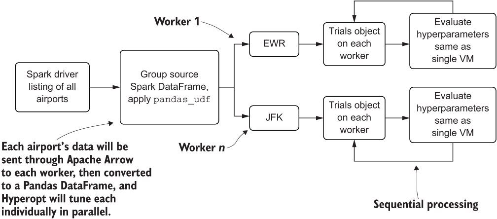
Figure 7.12 Using Spark to control a fleet of contained VMs to work on each forecast asynchronously
Here, we’re using Spark DataFrames—a distributed dataset based on resiliently distributed dataset (rdd) relations residing on different VMs—to control the grouping-by of our primary modeling key (in this case, our Airport_Code field). We then pass this aggregated state to a pandas_udf that will leverage Apache Arrow to serialize the aggregated data to workers as a pandas DataFrame. This creates a multitude of concurrent Python VMs that are all operating on their own airport’s data as if they were a single VM.
A trade-off exists here, though. To make this approach work, we need to change some things with our code. Listing 7.9 shows the first of these changes: a movement of the MLflow logging logic to within our minimization function, the addition of logging arguments to our function arguments, and the generation of the forecast plots for each iteration from within the minimization function so that we can see them after the modeling phase is completed.
Listing 7.9 Modifying the minimization function to support a distributed model approach
def hwes_minimization_function_udf(selected_hp_values, train, test, loss_metric,  airport, experiment_name, param_count, name, target_name, image_name, trial):                                                  ❶
    model_results = exp_smoothing_raw_udf(train, test, selected_hp_values)
    errors = calculate_errors(test, model_results['forecast'],
      extract_param_count_hwes(selected_hp_values))
    with mlflow.start_run(run_name='{}_{}_{}_{}'.format(airport,          ❷
        experiment_name,str(uuid.uuid4())[:8], len(trial.results))):
      mlflow.set_tag('airport', airport)                                  ❸
      mlflow.set_tag('parent_run', experiment_name)                       ❹
      mlflow.log_param('id', mlflow.active_run().info.run_id)             ❺
      mlflow.log_params(selected_hp_values)                               ❻
      mlflow.log_metrics(errors)                                           ❼
      img = plot_predictions(test,
                       model_results['forecast'],
                       param_count,
                       name,
                       target_name,
                       image_name)
      mlflow.log_artifact(image_name)                                     ❽
    return {'loss': errors[loss_metric], 'status': STATUS_OK}
❶ Adds arguments to support MLflow logging
❷ Initializes each iteration to its own MLflow run with a unique name to prevent collisions
❸ Adds searchable tags for the MLflow UI search functionality
❹ Searchable tags for the collection of all models that have been built for a particular execution of the job
❺ Records the iteration number of Hyperopt
❻ Records the hyperparameters for a particular iteration
❼ Logs the loss metrics for the iteration
❽ Saves the image (in PNG format) generated from the plot_predictions function that builds the test vs. forecast data
Since we’re going to be executing a pseudo-local Hyperopt run from directly within the Spark workers, we need to create our training and evaluation logic directly within a new function that will consume the grouped data passed via Apache Arrow to the workers for processing as a pandas DataFrame. The next listing shows the creation of this user-defined function (udf).
Listing 7.10 Creating the distributed model pandas_udf to build models concurrently
output_schema = StructType([
  StructField('date', DateType()),
  StructField('Total_Passengers_pred', IntegerType()),
  StructField('Airport', StringType()),
  StructField('is_future', BooleanType())
])                                                                        ❶

@pandas_udf(output_schema, PandasUDFType.GROUPED_MAP)                     ❷
def forecast_airports(airport_df):

  airport = airport_df['Airport_Code'][0]                                 ❸
  hpopt_space = {
    'model': {
          'trend': hp.choice('trend', ['add', 'mul']),
          'seasonal': hp.choice('seasonal', ['add', 'mul']),
          'seasonal_periods': hp.quniform('seasonal_periods', 12, 120, 12),
          'damped': hp.choice('damped', [True, False])
    },
    'fit': {
          'smoothing_level': hp.uniform('smoothing_level', 0.01, 0.99),
          'smoothing_seasonal': hp.uniform('smoothing_seasonal', 0.01, 0.99),
          'damping_slope': hp.uniform('damping_slope', 0.01, 0.99),
          'use_brute': hp.choice('use_brute', [True, False]),
          'use_boxcox': hp.choice('use_boxcox', [True, False]),
          'use_basinhopping': hp.choice('use_basinhopping', [True, False]),
          'remove_bias': hp.choice('remove_bias', [True, False])
    }
  }                                                                       ❹

  run_config = {'minimization_function': hwes_minimization_function_udf,
                  'tuning_space': hpopt_space,
                  'forecast_algo': exp_smoothing_raw,
                  'loss_metric': 'bic',
                  'hpopt_algo': tpe.suggest,
                  'iterations': 200,
                  'experiment_name': RUN_NAME,
                  'name': '{} {}'.format('Total Passengers HPOPT', airport),
                  'target_name': 'Total_Passengers',
                  'image_name': '{}_{}.png'.format('total_passengers_               validation', airport),
                  'airport_name': airport,
                  'future_forecast_periods': 36,
                  'train_split_cutoff_months': 12,
                  'hyperopt_title': '{}_hyperopt Training
                    Report'.format(airport),
                  'hyperopt_image_name': '{}_{}.png'.format(
                    'total_passengers_hpopt', airport),
                  'verbose': True
            }                                                             ❺


  airport_data = airport_df.copy(deep=True)
  airport_data['date'] = pd.to_datetime(airport_data['date'])
  airport_data.set_index('date', inplace=True)
  airport_data.index = pd.DatetimeIndex(airport_data.index.values, freq=airport_data.index.inferred_freq)
  asc = airport_data.sort_index()
  asc = apply_index_freq(asc, 'MS')                                       ❻

  train, test = generate_splits_by_months(asc, run_config['train_split_cutoff_months'])

  tuning = run_udf_tuning(train['Total_Passengers'], test['Total_Passengers'], **run_config)                              ❼

  return tuning                                                           ❽
❶ Since Spark is a strong-typed language, we need to provide expectations to the udf of what structure and data types pandas will be returning to the Spark DataFrame. This is accomplished by using a StructType object defining the field names and their types.
❷ Defines the type of the pandas_udf (here we are using a grouped map type that takes in a pandas DataFrame and returns a pandas DataFrame) through the decorator applied above the function
❸ We need to extract the airport name from the data itself since we can’t pass additional values into this function.
❹ We need to define our search space from within the udf since we can’t pass it into the function.
❺ Sets the run configuration for the search (within the udf, since we need to name the runs in MLflow by the airport name, which is defined only after the data is passed to a worker from within the udf)
❻ The airport data manipulation of the pandas DataFrame is placed here since the index conditions and frequencies for the series data are not defined within the Spark DataFrame.
❼ The only modification to the “run tuning” function is to remove the MLflow logging created for the driver-based distributed Hyperopt optimization and to return only the forecasted data instead of the dictionary containing the run metrics and data.
❽ Returns the forecast pandas DataFrame (required so that this data can be “reassembled” into a collated Spark DataFrame when all the airports finish their asynchronous distributed tuning and forecast runs)
With the creation of this pandas_udf, we can call the distributed modeling (using Hyperopt in its single-node Trials() mode).
Listing 7.11 Executing a fully distributed model-based asynchronous run of forecasting
def validate_data_counts_udf(data, split_count):                           ❶
    return (list(data.groupBy(col('Airport_Code')).count()
          .withColumn('check', when(((lit(12) / 0.2) < (col('count') * 0.8)),
            True)
          .otherwise(False))
          .filter(col('check')).select('Airport_Code').toPandas()[             'Airport_Code']))

RUN_NAME = 'AIRPORT_FORECAST_DEC_2020'                                     ❷
raw_data = spark.table(delta_full_nm)                                      ❸
filtered_data = raw_data.where(col('Airport_Code').isin(validate_data_counts_udf(raw_data, 12))).repartition('Airport_Code')                               ❹
grouped_apply = filtered_data.groupBy('Airport_Code').apply(forecast_airports)        ❺
display(grouped_apply)                                                     ❻
❶ A modification of the airport filtering used in the single-node code, utilizing PySpark filtering to determine whether enough data is in a particular airport’s series to build and validate a forecasting model
❷ Defines a unique name for the particular execution of a forecasting run (this sets the name of the MLflow experiment for the tracking API)
❸ Reads the data from Delta (raw historical passenger data for airports) into the workers on the cluster
❹ Filters out insufficient data wherein a particular airport does not have enough data for modeling
❺ Groups the Spark DataFrame and sends the aggregated data to the workers as pandas DataFrames for execution through the udf
❻ Forces the execution (Spark is lazily evaluated)
When we run this code, we can see a relatively flat relationship between the number of airport models being generated and the number of workers available for processing our optimization and forecasting runs. While the reality of modeling over 7,000 airports in the shortest amount of time (a Spark cluster with thousands of worker nodes) is more than a little ridiculous (the cost alone would be astronomical), we have a queue-able solution using this paradigm that can horizontally scale in a magnitude that any other solution cannot.
Even though we wouldn’t be able to get an effective O(1) execution time because of cost and resources (that would require one worker for each model), we can start a cluster with 40 nodes that would, in effect, run 40 airport modeling, optimizing, and forecasting executions concurrently. This would dramatically reduce the total runtime to 23 hours for all 7,000 airports, as opposed to either running them in a VM through a sequential loop-within-a-loop (> 5,000 hours), or collecting the data to the driver of a Spark cluster and running distributed tuning (> 800 hours).
When finding options for tackling large-scale projects of this nature, the scalability of the execution architecture is just as critical as any of the ML components. Regardless of how much effort, time, and diligence went into crafting the ML aspect of the solution, if solving the problem takes thousands (or hundreds) of hours, the chances that the project will succeed are slim. In the next chapter, section 8.2, we will discuss alternative approaches that can reduce the already dramatically improved 23 hours of runtime down to something even more manageable.
7.2.4 Using new paradigms for teams: Platforms and technologies
Starting on a new platform, utilizing a new technology, and perhaps learning a new programming language (or paradigm within a language you already know) is a daunting task for many teams. In the preceding scenarios, it was a relatively large leap to move from a Jupyter notebook running on a single machine to a distributed execution engine like Spark.
The world of ML provides a great many options—not only in algorithms, but also in programming languages (R, Python, Java, Scala, .NET, proprietary languages) and places to develop code (notebooks for prototyping, scripting tools for MVPs, and IDEs for production solution development). Most of all, a great many places are available to run the code that you’ve written. As we saw earlier, it wasn’t the language that caused the runtime of the project to drop so dramatically, but rather the platform that we chose to use.
When exploring options for project work, it is absolutely critical to do your homework. It is critical to test different algorithm approaches to solve a particular problem, and it is arguably more critical to find a place to run the solutions that fits within the needs of that project.
To maximize the chances of a solution being adopted by the business, the right platform should be chosen to minimize execution cost, maximize the stability of the solution, and shorten the development cycle to meet delivery deadlines. The important point to keep in mind about where to run ML code is that it is like any other aspect of this profession: time spent learning the framework used to run your models and analyses will be well spent, enhancing your productivity and efficiency for future work. Without knowing how to actually use a particular platform or execution paradigm, as mentioned in section 7.2.3, this project could have been looking at hundreds of hours of runtime for each forecasting event initiated.
Summary
- Relying on manual and prescriptive approaches for model tuning is time-consuming, expensive, and unlikely to produce quality results. Utilizing model-driven parameter optimization is preferred.
- Selecting an appropriate platform and implementation methodology for time-consuming CPU-bound tasks can dramatically increase the efficiency and lower the cost of development for an ML project. For processes like hyperparameter tuning, maximizing parallel and distributed system approaches can reduce the development timeline significantly.