
Appendix A. Big O(no) and how to think about runtime performance
Runtime complexity, for ML use cases, is no different than it is for any other piece of software. The impact of inefficient and poorly optimized code affects processing tasks in ML jobs the same as it does any other engineering project. The only material difference that sets ML tasks apart from traditional software is in the algorithms employed to solve problems. The computational and space complexity of these algorithms is typically obscured by high-level APIs that encapsulate recursive iterations, which can dramatically increase runtimes.
The goal of this appendix is to focus on understanding both the runtime characteristics of control code (all the code in your project that isn’t involved in training a model) and the ML algorithm itself that is being trained.
A.1 What is Big O, anyway?
Let’s suppose we’re working on a project that is set to release soon to production. The results are spectacular, and the business unit for whom the project was built is happy with the attribution results. However, not everyone is happy. The costs of running the solution are incredibly high.
As we step through the code, we discover that the vast majority of the execution time is centered around our feature-engineering preprocessing stages. One particular portion of the code seems to take far longer than we originally expected. Based on initial testing, shown in the following listing, we had imagined that this function wouldn’t be much of a problem.
Listing A.1 Nested loop name-reconciliation example
import nltk
import pandas as pd
import numpy as np
client_names = ['Rover', 'ArtooDogTwo', 'Willy', 'Hodor',
  'MrWiggleBottoms', ‘SallyMcBarksALot', 'HungryGames',
  'MegaBite', 'HamletAndCheese', 'HoundJamesHound',
  'Treatzilla', 'SlipperAssassin', 'Chewbarka',
  'SirShedsALot', 'Spot', 'BillyGoat', 'Thunder',
  'Doggo', 'TreatHunter']                                      ❶
extracted_names = ['Slipr Assassin', 'Are two dog two',
  'willy', 'willie', 'hodr', 'hodor', 'treat zilla',
  'roover', 'megbyte', 'sport', 'spotty', 'billygaot',
  'billy goat', 'thunder', 'thunda', 'sirshedlot',
  'chew bark', 'hungry games', 'ham and cheese',
  'mr wiggle bottom', 'sally barks a lot']                     ❷
def lower_strip(string): return string.lower().replace(" ", "")
def get_closest_match(registered_names, extracted_names):
    scores = {}
    for i in registered_names:                                 ❸
        for j in extracted_names:                              ❹
            scores['{}_{}'.format(i, j)] = nltk.edit_distance(lower_strip(i),
       lower_strip(j))                                         ❺
    parsed = {}
    for k, v in scores.items():                                ❻
        k1, k2 = k.split('_')
        low_value = parsed.get(k2)
        if low_value is not None and (v < low_value[1]):
            parsed[k2] = (k1, v)
        elif low_value is None:
            parsed[k2] = (k1, v)
    return parsed
get_closest_match(client_names, extracted_names)               ❼
>> {'Slipr Assassin': ('SlipperAssassin', 2),
    'Are two dog two': ('ArtooDogTwo', 2),
    'willy': ('Willy', 0),
    'willie': ('Willy', 2),
    'hodr': ('Hodor', 1),
    'hodor': ('Hodor', 0),
    'treat zilla': ('Treatzilla', 0),
    'roover': ('Rover', 1),
    'megbyte': ('MegaBite', 2),
    'sport': ('Spot', 1),
    'spotty': ('Spot', 2),
    'billygaot': ('BillyGoat', 2),
    'billy goat': ('BillyGoat', 0),
    'thunder': ('Thunder', 0),
    'thunda': ('Thunder', 2),
    'sirshedlot': ('SirShedsALot', 2),
    'chew bark': ('Chewbarka', 1),
    'hungry games': ('HungryGames', 0),
    'ham and cheese': ('HamletAndCheese', 3),
    'mr wiggle bottom': ('MrWiggleBottoms', 1),
    'sally barks a lot': ('SallyMcBarksALot', 2)}              ❽
❶ The list of registered names of dogs in our database (small sample)
❷ The parsed names from the free-text field ratings that we get from our customer’s humans
❸ Looping through every one of our registered names
❹ The O(n2) nested loop, going through each of the parsed names
❺ Calculates the Levenshtein distance between the names after removing spaces and forcing lowercase on both strings
❻ Loops through the pairwise distance measurements to return the most likely match for each parsed name. This is O(n).
❼ Runs the algorithm against the two lists of registered names and parsed names
❽ The results of closest match by Levenshtein distance
On the small dataset used for validation and development, the execution time was in milliseconds. However, when running against our full dataset of 5 million registered dogs and 10 billion name reference extractions, we simply have too many dogs in our data to run through this algorithm. (Yes, there can be such a thing as too many dogs, believe it or not.).
The reason is that the computational complexity of this algorithm is O(n2). For each registered name, we’re testing its distance to each of the name extracts, as shown in figure A.1.
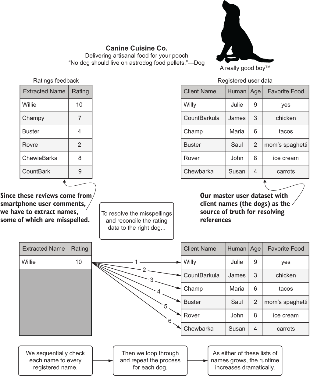
Figure A.1 The computational complexity of our feature engineering
The following listing shows an alternative approach to reducing the looped searching.
Listing A.2 A slightly better approach (but still not perfect)
JOIN_KEY = 'joinkey'
CLIENT_NM = 'client_names'
EXTRACT_NM = 'extracted_names'
DISTANCE_NM = 'levenshtein'

def dataframe_reconciliation(registered_names, extracted_names, threshold=10):
    C_NAME_RAW = CLIENT_NM + '_raw'
    E_NAME_RAW = EXTRACT_NM + '_raw'
    registered_df = pd.DataFrame(registered_names, columns=[CLIENT_NM])     ❶
    registered_df[JOIN_KEY] = 0                                             ❷
    registered_df[C_NAME_RAW] = registered_df[CLIENT_NM].map(lambda x: lower_strip(x))                                                        ❸
    extracted_df = pd.DataFrame(extracted_names, columns=[EXTRACT_NM])
    extracted_df[JOIN_KEY] = 0                                              ❹
    extracted_df[E_NAME_RAW] = extracted_df[EXTRACT_NM].map(lambda x: lower_strip(x))
    joined_df = registered_df.merge(extracted_df, on=JOIN_KEY, how='outer') ❺
    joined_df[DISTANCE_NM] = joined_df.loc[:, [C_NAME_RAW, E_NAME_RAW]].apply(
        lambda x: nltk.edit_distance(*x), axis=1)                           ❻
    joined_df = joined_df.drop(JOIN_KEY, axis=1)
    filtered = joined_df[joined_df[DISTANCE_NM] < threshold]                ❼
    filtered = filtered.sort_values(DISTANCE_NM).groupby(EXTRACT_NM, as_index=False).first()                                                ❽
    return filtered.drop([C_NAME_RAW, E_NAME_RAW], axis=1)
❶ Creates a pandas DataFrame from the client names list
❷ Generates a static join key to support our Cartesian join we’ll be doing
❸ Cleans up the names so that our Levenshtein calculation can be as accurate as possible (function defined in listing A.1)
❹ Generates the same static join key in the right-side table to effect the Cartesian join
❺ Performs the Cartesian join (which is O(n2) space complexity)
❻ Calculates the Levenshtein distance by using the thoroughly useful NLTK package
❼ Removes any potential non-matches from the DataFrame
❽ Returns the rows for each potential match key that has the lowest Levenshtein distance score
NOTE if you’re curious about the NLTK package and all of the fantastic things that it can do for natural language processing in Python, I highly encourage you to read Natural Language Processing with Python (O’Reilly, 2009) by Steven Bird, Ewan Klein, and Edward Loper, the original authors of the open source project.
Utilizing this DataFrame approach can remarkably speed up the runtime. Listing A.2 is not a perfect solution, since the space complexity will increase, but refactoring in this manner can dramatically reduce the runtime of the project and reduce costs. Figure A.2 shows the results of calling the function defined in listing A.2.
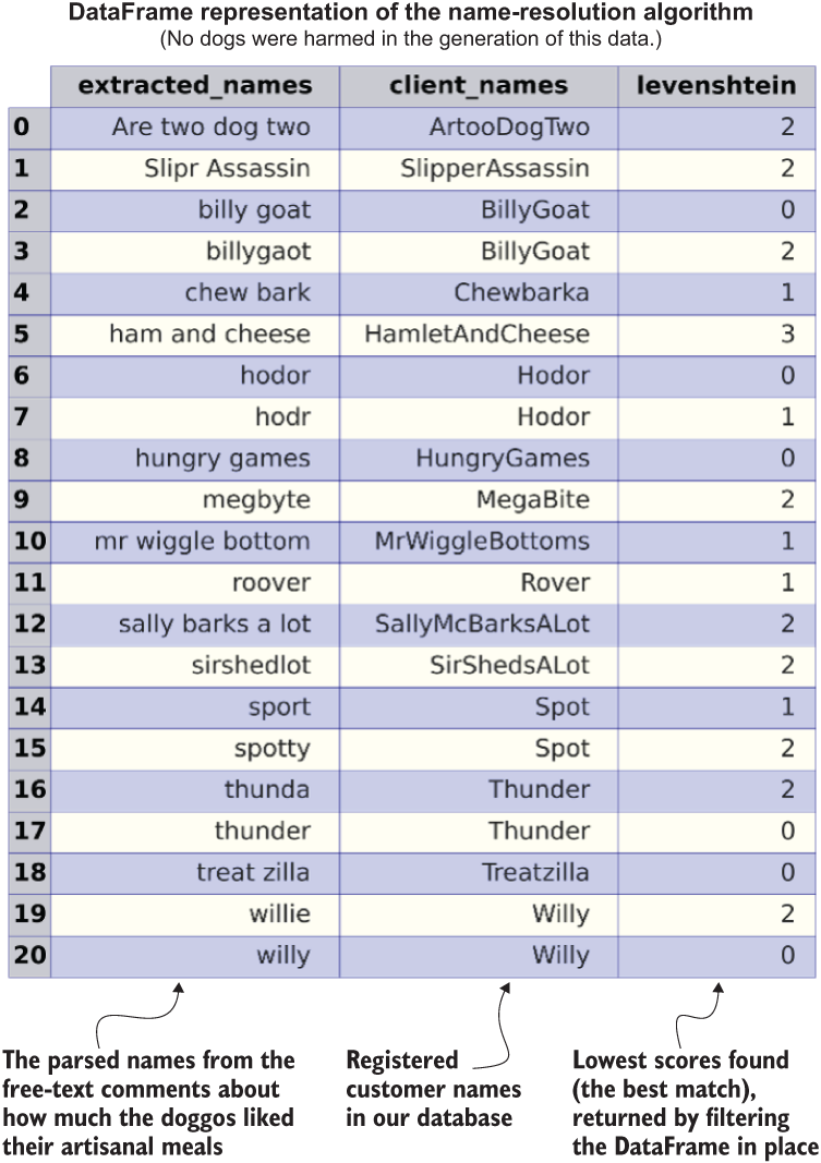
Figure A.2 Reducing computational complexity at the expense of space complexity
The important thing to remember about this example is that scalability is relative. Here we are trading computational complexity for space complexity: we originally were sequentially looping through two arrays, which takes a long time to do, but has a very low memory footprint; then, working with the matrix-like structure of pandas is orders of magnitude faster but requires a great deal of RAM. In actual practice, with the data volumes involved here, the best solution is to process this problem in a mix of looped processing (preferably in Spark DataFrame s) while leveraging Cartesian joins in chunks to find a good balance between computation and space pressure.
The analysis of runtime issues is, from both a practical and theoretical stance, handled through evaluating computational complexity and space complexity, referred to in shorthand as Big O.
A.1.1 A gentle introduction to complexity
Computational complexity is, at its heart, a worst-case estimation of how long it will take for a computer to work through an algorithm. Space complexity, on the other hand, is the worst-case burden to a system’s memory that an algorithm can cause.
While computational complexity typically impacts the CPU, space complexity involves the memory (RAM) you need to have in the system to process the algorithm without incurring disk spills (pagination to a hard drive or solid-state drive). Figure A.3 shows how operating on a collection of data points can have different space and computational complexity, depending on the algorithm that you’re using.
The different actions being performed on collections of data affect the amount of time and space complexity involved. As you move from top to bottom in figure A.3, both space and computational complexity increase for different operations.
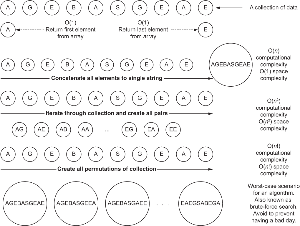
Figure A.3 Comparison of computational and space complexities for operating on a collection of data
Many other complexities are considered standard for assessing complexities in algorithms. Figure A.4 shows these standard assessments on a linear scale, while figure A.5 shows them on a logarithmic y-scale to illustrate just how much some of them should be avoided.
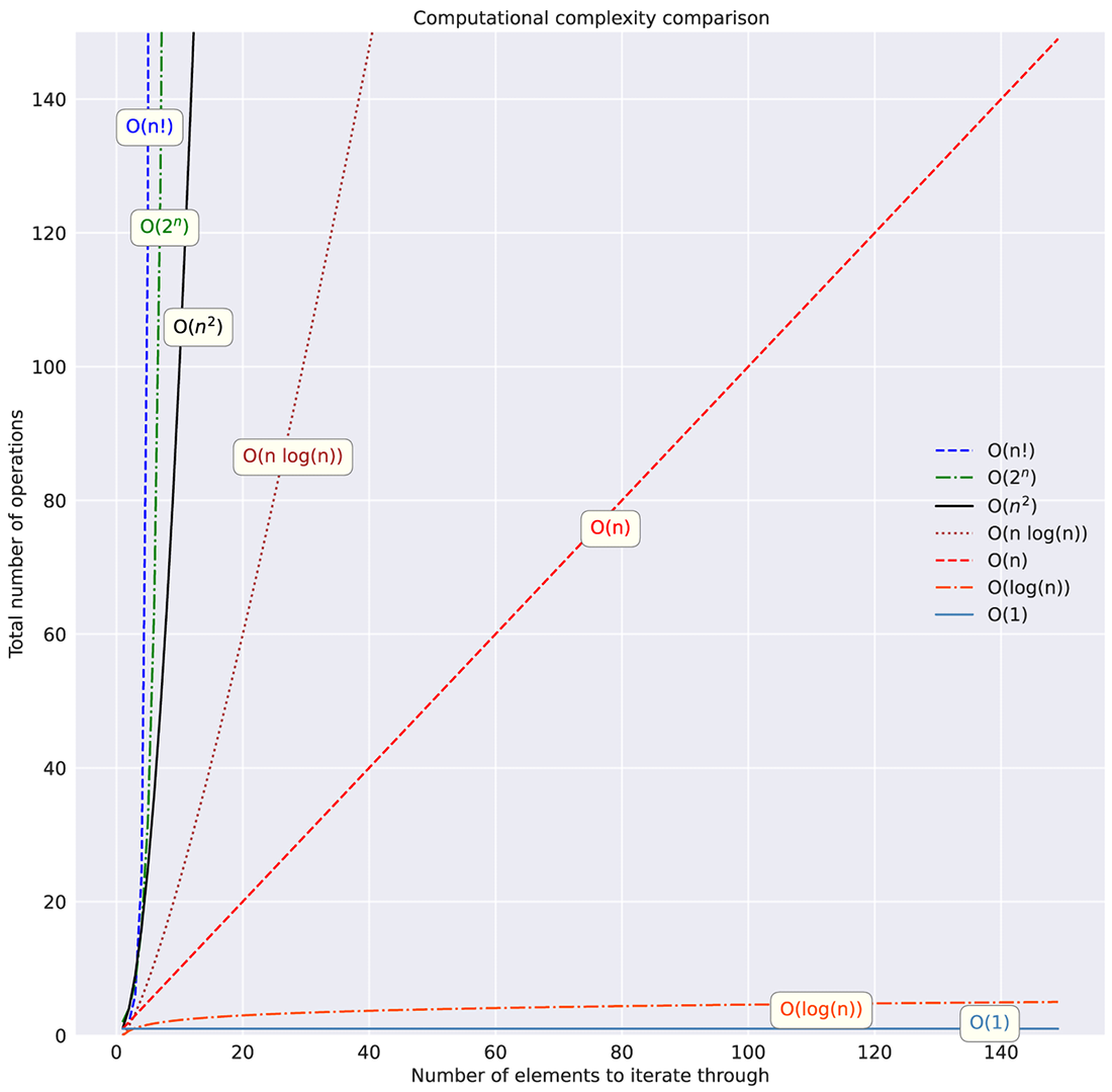
Figure A.4 Linear y-axis scale of different computational complexities filtered to 150 iterations
As figures A.4 and A.5 show, the relationship between collection size and algorithm type can dramatically affect the runtime of your code. Understanding these relationships (of both space and computational complexity) within the non-ML aspects of your code, outside of model training and inference, is absolutely essential.
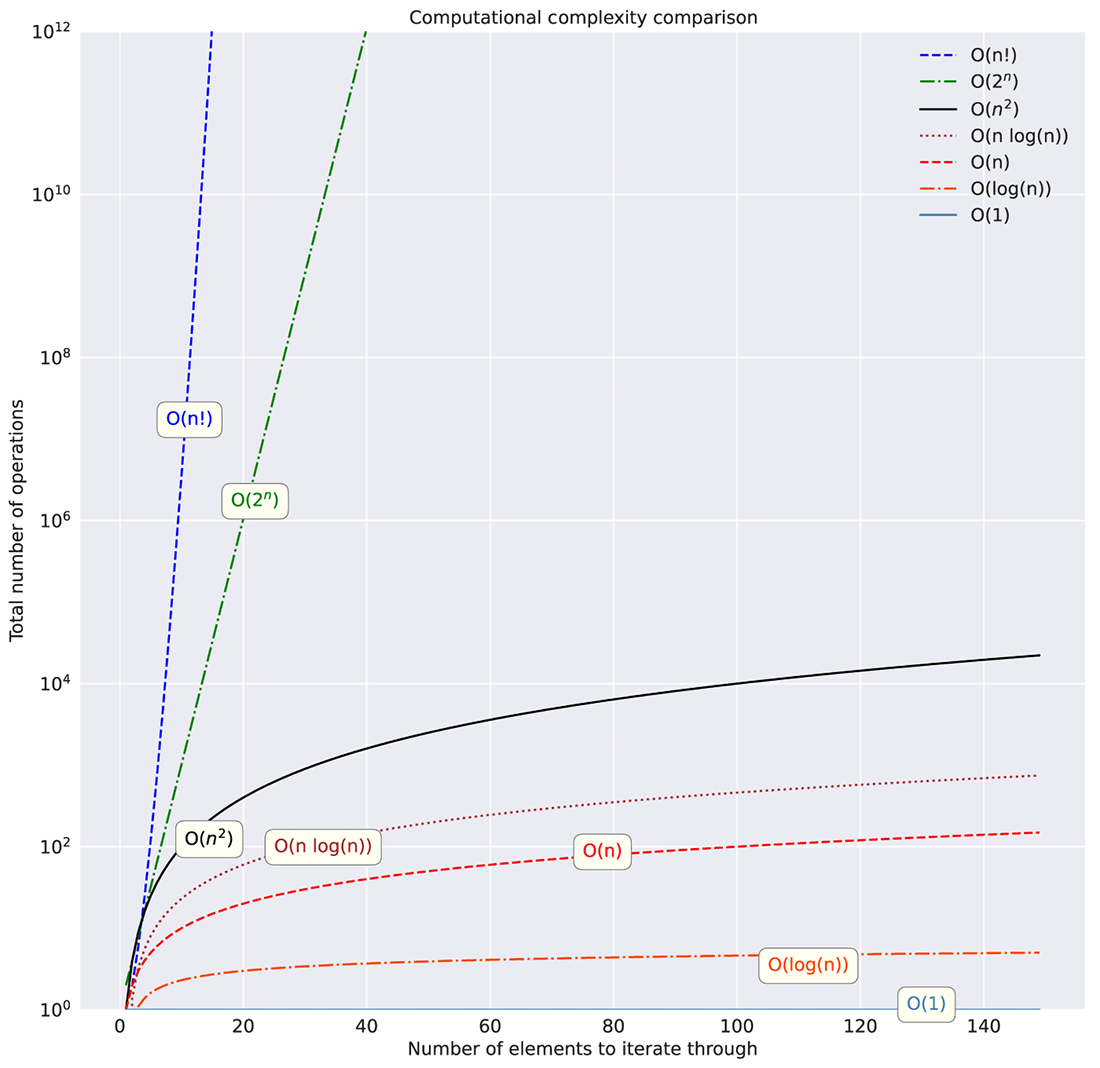
Figure A.5 Logarithmic y-axis scale of computational complexities. Pay close attention to the size of the y-axis toward the top of the graph. Exponential and factorial complexities can truly bring the pain.
Let’s imagine what the costs would be for implementing something as simple as a collection traversal in project orchestration code. If we were trying to evaluate relationships between two arrays of numbers in a brute-force manner (looping through each in a nested fashion), we’d be looking at O(n2) complexity. If we were to merge the lists instead through an optimized join, we could reduce the complexity significantly. Moving from complexities like O(n2) to something closer to O(n), as shown in figures A.4 and A.5, when dealing with large collections, can translate to significant cost and time savings.
A.2 Complexity by example
Analyzing code for performance issues can be daunting. Many times, we’re so focused on getting all of the details surrounding feature engineering, model tuning, metric evaluation, and statistical evaluation ironed out that the concept of evaluating how we’re iterating over collections doesn’t enter our minds.
If we were to take a look at the control code that directs the execution of those elements of a project, thinking of their execution as a factor of complexity, we would be able to estimate the relative runtime effects that will occur. Armed with this knowledge, we could decouple inefficient operations (such as overly nested looping statements that could be collapsed into a single indexed traversal) and help reduce the burden on both the CPU and the memory of the system running our code.
Now that you’ve seen the theory of Big O, let’s take a look at some code examples using these algorithms. Being able to see how differences in the number of elements in a collection can affect timing of operations is important in order to fully understand these concepts.
I’m going to present these topics in a somewhat less-than-traditional manner, using dogs as an example, followed by showing code examples of the relationships. Why? Because dogs are fun.
A.2.1 O(1): The “It doesn’t matter how big the data is” algorithm
Let’s imagine that we’re in a room. A very, very large room. In the center of the room is a ring of food bowls. For dogs. And we’ve filled these bowls with some pasta Bolognese. It’s been a torturous day of making it (for the dogs, smelling the entire time), but we’ve ladled the food into five separate bowls and are ready with our notepads to record data about the event. After all is said and done (bowls are cleaner than before they were ladled with pasta), we have collections of ordered lists representing different actions that our panel of dogs took.
When we wish to answer questions about the facts that we observed, we’re operating on these lists, but retrieving a single indexed value associated with the order in which these events occurred. Regardless of the size of these lists, the O(1)-type questions are simply acquiring data based on positional reference, and thus, the operations all take the same amount of time. Let’s take a look at this scenario in figure A.6.
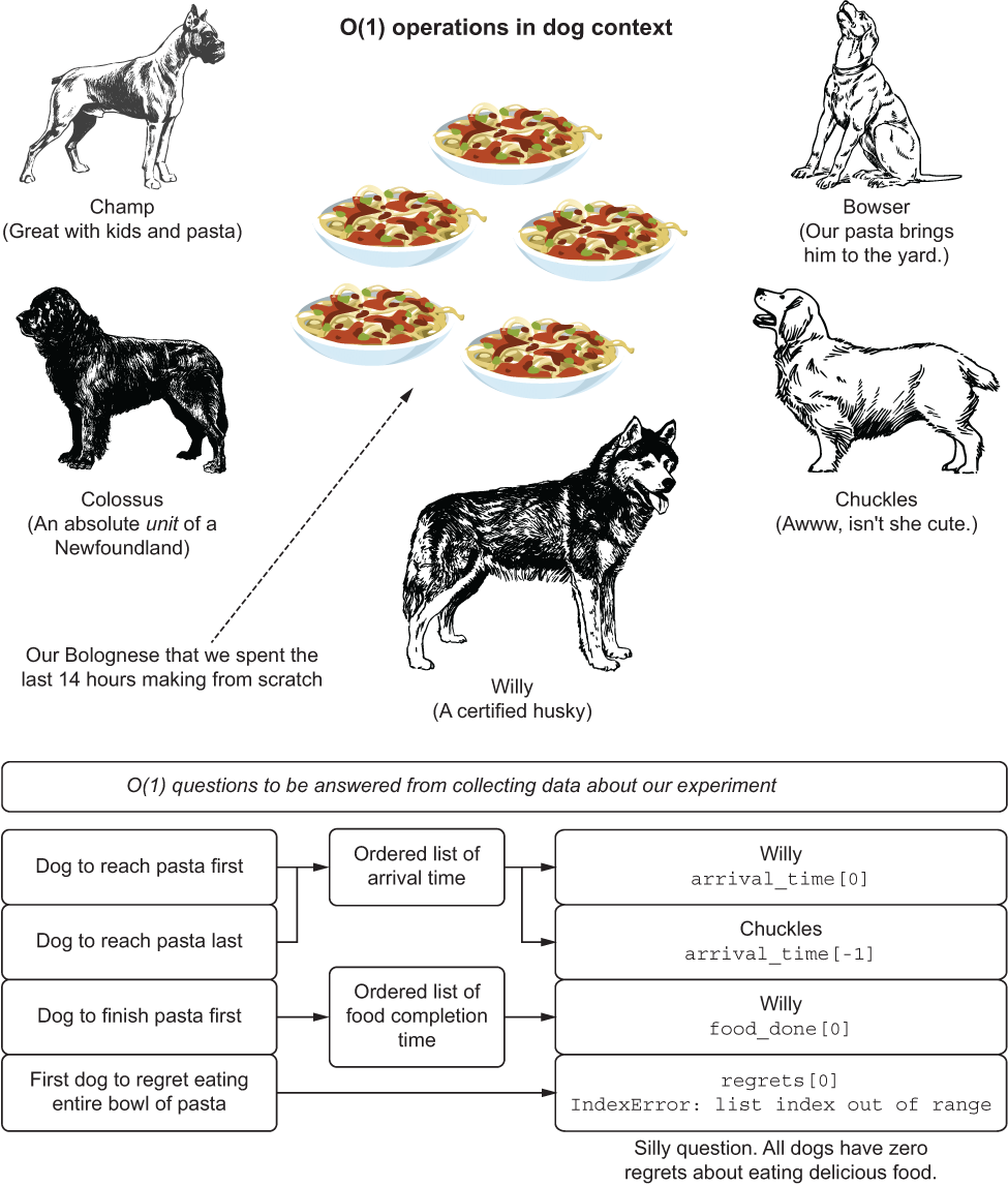
Figure A.6 O(1) search by means of hungry dogs
O(1) doesn’t care how big the data is, as figure A.6 shows. These algorithms simply operate in ways that don’t traverse collections, but rather access positions of data within collections.
To show this relationship in a computational sense, listing A.3 illustrates a comparison of performing an O(1) task on two differently sized collections of data—with a similar runtime performance.
Listing A.3 Demonstration of O(1) complexity
import numpy as np
sequential_array = np.arange(-100, 100, 1)                     ❶
%timeit -n 1000 -r 100 sequential_array[-1]                    ❷
>> 269 ns ± 52.1 ns per loop (mean ± std. dev. of
100 runs, 10000 loops each)                                    ❸
massive_array = np.arange(-1e7, 1e7, 1)                        ❹
%timeit -n 10000 -r 100 massive_array[-1]
>> 261 ns ± 49.7 ns per loop (mean ± std. dev. of
100 runs, 10000 loops each)                                    ❺
def quadratic(x):                                              ❻
    return (0.00733 * math.pow(x, 3) -0.001166 *
math.pow(x, 2) + 0.32 * x - 1.7334)
%timeit -n 10000 -r 100 quadratic(sequential_array[-1])        ❼
>> 5.31 µs ± 259 ns per loop (mean ± std. dev. of 100 runs, 10000 loops each)
%timeit -n 10000 -r 100 quadratic(massive_array[-1])           ❽
>> 1.55 µs ± 63.3 ns per loop (mean ± std. dev. of 100 runs, 10000 loops each)
❶ Generates an array of integers between -100 and 100
❷ Runs through 100,000 iterations of the operation to allow for per-run variance to be minimized to see the access speed
❸ The absolute value of average speed per iteration is highly dependent on the hardware that the code is running on. 269 nanoseconds is pretty fast for using a single core from an 8-core laptop CPU, though.
❹ Generates an array that is just slightly larger than the first one
❺ 261 nanoseconds. Even with 100,000 times more data, the execution time is the same.
❻ Quadratic equation to illustrate mathematical operations on a single value
❼ Executes 5.31 microseconds on a single value from the array
❽ Executes 1.55 microseconds on a single value from the array (less time than the previous due to indexing operations in NumPy for accessing larger arrays)
The first array (sequential_array) is a scant 200 elements in length, and its access time for retrieving an element from its indexed c-based-struct type is very fast. As we increase the size of the array (massive_array, containing 2 million elements), the runtime doesn’t change for a positional retrieval. This is due to an optimized storage paradigm of the array; we can directly look up the memory address location for the element in constant O(1) time through the index registry.
The control code of ML projects has many examples of O(1) complexity:
- Getting the last entry in a sorted, ranked collection of aggregated data points—For example, from a window function with events arranged by time of occurrence. However, the process of building the windowed aggregation is typically O(n log n) because of the sort involved.
- A modulo function—This indicates the remainder after dividing one number by another and is useful in pattern generation in collection traversals. (The traversal will be O(n), though.)
- Equivalency test—Equal, greater than, less than, and so forth.
A.2.2 O(n): The linear relationship algorithm
What if we want to know the status of our canine test subjects at a particular point in time? Let’s say that we really want to find out the rate at which they are wolfing down their food. Suppose that we decide to collect data at 30 seconds into the feast to see the state of the food bowls for each dog.
The data that we collect for each dog would involve a key-value pairing. In Python, we would be collecting a dictionary containing the names of the dogs and the amount of food remaining in their bowls:
thirty_second_check = {'champ': 0.35, 'colossus': 0.65,
    'willy': 0.0, 'bowser': 0.75, 'chuckles': 0.9}
This operation, walking around and estimating the amount of food left in the bowls, recording it in this (key, value) pairing, would be O(n), as illustrated in figure A.7.
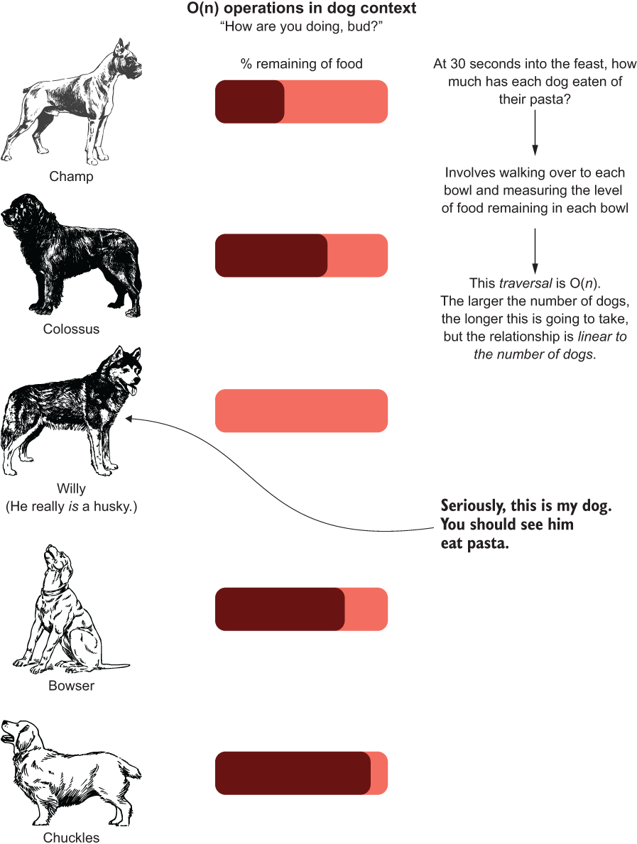
Figure A.7 O(n) search through all of the dogs’ consumption rates
As you can see, in order to measure the amount remaining, we need to walk around to each dog and check the state of their bowl. For the five dogs we’re showing, that may take a few seconds. But what if we had 500 dogs? That would take a few minutes of walking around to measure. The O(n) indicates a linear relationship between the algorithm (checking the amount of Bolognese eaten) and the size of the data (number of dogs) as a reflection of computational complexity.
From a software perspective, the same relationship holds true. Listing A.4 shows an iterative usage of the quadratic() method defined in listing A.3, operating over each element in the two NumPy arrays defined in that listing. As the size of the array increases, the runtime increases in a linear manner.
Listing A.4 Demonstration of O(n) complexity
%timeit -n 10 -r 10 [quadratic(x) for x in sequential_array]
>> 1.37 ms ± 508 µs per loop (mean ± std. dev. of 10 runs, 10 loops each)  ❶
%timeit -n 10 -r 10 [quadratic(x) for x in np.arange(-1000, 1000, 1)]
>> 10.3 ms ± 426 µs per loop (mean ± std. dev. of 10 runs, 10 loops each)  ❷
%timeit -n 10 -r 10 [quadratic(x) for x in np.arange(-10000, 10000, 1)]
>> 104 ms ± 1.87 ms per loop (mean ± std. dev. of 10 runs, 10 loops each)  ❸
%timeit -n 10 -r 10 [quadratic(x) for x in np.arange(-100000, 100000, 1)]
>> 1.04 s ± 3.77 ms per loop (mean ± std. dev. of 10 runs, 10 loops each)
%timeit -n 2 -r 3 [quadratic(x) for x in massive_array]
>> 30 s ± 168 ms per loop (mean ± std. dev. of 3 runs, 2 loops each)       ❹
❶ Mapping over the small (-100, 100) array and applying a function to each value takes a bit longer than retrieving a single value.
❷ Increases the size by a factor of 10 for the array, and the runtime increases by a factor of 10
❸ Increases again by a factor of 10, and the runtime follows suit. This is O(n).
❹ Increases by a factor of 10, and the runtime increases by a factor of 30?! This is due to the size of the values being calculated and the shift to an alternative form of multiplication in Cython (the underlying compiled C* code that optimized calculations use).
As can be seen in the results, the relationship between collection size and computational complexity is for the most part relatively uniform(see the following callout for why it’s not perfectly uniform here).
O(n) is a fact of life in our world of DS work. However, we should all pause and reconsider our implementations if we’re building software that employs our next relationship in this list: O(n2). This is where things can get a little crazy.
A.2.3 O(n2): A polynomial relationship to the size of the collection
Now that our dogs are fed, satiated, and thoroughly pleased with their meal, they could use a bit of exercise. We take them all to a dog park and let them enter at the same time.
As in any social hour involving dogs, the first order of business is going to be formal introductions by way of behind-sniffing. Figure A.8 shows the combinations of greetings among our five dogs.
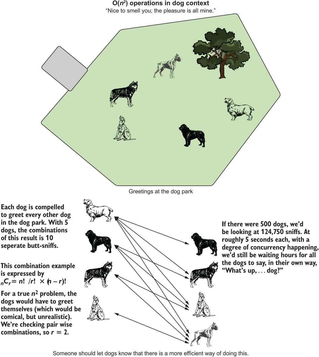
Figure A.8 The dog park meet and greet. While not precisely O(n2), it bears a similar relationship.
NOTE Combination calculations are, in the strictest sense, O(n choose k) in complexity. For simplicity’s sake, let’s imagine brute-forcing the solution by interacting all possible permutations and then filtering, which would be O(n2) in complexity.
This combination-based traversal of paired relationships is not strictly O(n2); it is actually O(n choose k). But we can apply the concept and show the number of operations as combinatorial operations. Likewise, we can show the relationship between runtime duration and collection size by operating on permutations
Table A.1 shows the number of total butt-sniff interactions that will happen in this dog park based on the number of dogs let in through the gate (combinations), as well as the potential greetings. We’re assuming the dogs feel the need for a formal introduction, wherein each acts as the initiator (a behavior that I have witnessed with my dog on numerous occasions).
Table A.1 Dog greeting by number of dogs
To illustrate what this relationship of friendly dog greetings looks like for both the combinations and permutations, figure A.9 shows the incredible growth in complexity as the number of dogs increases.
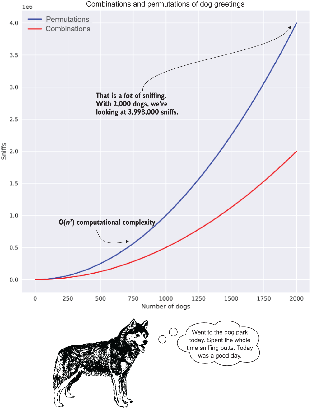
Figure A.9 The explosion of sniffing as the number of dogs increases in our dog park. Exponential relationships in complexity are just as bad in code as they are for dogs when talking about efficiency.
For the vast majority of ML algorithms (the models that are built through a training process), this level of computational complexity is just the beginning. Most are far more complex than O(n 2).
Listing A.5 shows an implementation of n 2 complexity. For each element of the source array, we’re going to be generating an offset curve that rotates the element by the iteration index value. The visualizations for each section following will show what is going on in the code to make it clearer.
Listing A.5 An example of O(n2) complexity
import seaborn as sns
def quadratic_div(x, y):                                                   ❶
    return quadratic(x) / y
def n_squared_sim(size):                                                   ❷
    max_value = np.ceil(size / 2)
    min_value = max_value * -1
    x_values = np.arange(min_value, max_value + 1, 1)                      ❸
    with warnings.catch_warnings():
        warnings.simplefilter("ignore")                                    ❹
        curve_matrix = [[quadratic_div(x, y) for x in x_values] for
                         y in x_values]                                    ❺
    curve_df = pd.DataFrame(curve_matrix).T
    curve_df.insert(loc=0, column='X', value=x_values)
    curve_melt = curve_df.melt('X', var_name='iteration', value_name='Y')  ❻
    fig = plt.figure(figsize=(10,10))
    ax = fig.add_subplot(111)
    sns.lineplot(x='X', y='Y', hue='iteration', data=curve_melt, ax=ax)    ❼
    plt.ylim(-100,100)
    for i in [ax.title, ax.xaxis.label, ax.yaxis.label] + ax.get_xticklabels() + ax.get_yticklabels():
        i.set_fontsize(14)
    plt.tight_layout
    plt.savefig('n_squared_{}.svg'.format(size), format='svg')
    plt.close()
    return curve_melt
❶ Function for modifying the quadratic solution to the array by a value from the array
❷ Function for generating the collection of quadratic evaluation series values
❸ Acquires the range around 0 for array generation (size + 1 for symmetry)
❹ Catches warnings related to dividing by zero (since we’re crossing that boundary of integers in the array)
❺ The n2 traversal to generate the array of arrays by mapping over the collection twice
❻ Transposes and melts the resultant matrix of data to a normalized form for plotting purposes
❼ Plots each curve with a different color to illustrate the complexity differences in the algorithm
For the algorithm defined in listing A.5, if we were to call it with different values for an effective collection size, we would get the timed results shown in the next listing.
Listing A.6 Results of evaluating an O(n2) complex algorithm
%timeit -n 2 -r 2 ten_iterations = n_squared_sim(10)
>> 433 ms ± 50.5 ms per loop (mean ± std. dev. of 2 runs, 2 loops each)   ❶
%timeit -n 2 -r 2 one_hundred_iterations = n_squared_sim(100)
>> 3.08 s ± 114 ms per loop (mean ± std. dev. of 2 runs, 2 loops each)    ❷
%timeit -n 2 -r 2 one_thousand_iterations = n_squared_sim(1000)
>> 3min 56s ± 3.11 s per loop (mean ± std. dev. of 2 runs, 2 loops each)  ❸
❶ With only 121 operations, this executes pretty quickly.
❷ At 10 times the array size, 10,201 operations take significantly longer.
❸ At 1,002,001 operations, the exponential relationship becomes clear.
The relationship to the input array size from listing A.5 and the results shown in listing A.6 can be seen a bit more clearly in figure A.10. If we were to continue increasing the size of the array generation parameter value to 100,000, we would be looking at 10,000,200,001 operations (while our first iteration of size 10 generates 121 operations). More important, though, is the memory pressure of generating so many arrays of data. The size complexity will rapidly become the limiting factor here, resulting in an out-of-memory (OOM) exception long before we get annoyed at how long it’s taking to calculate.
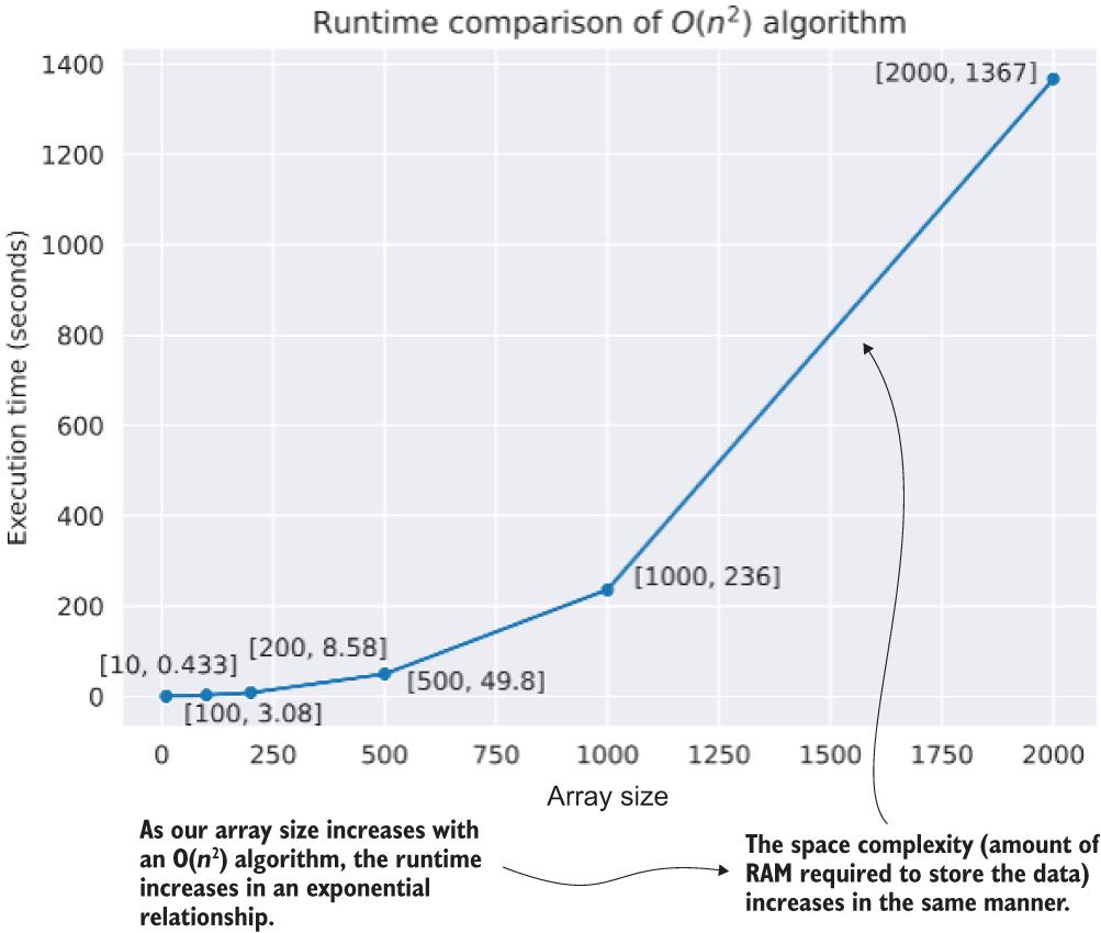
Figure A.10 Computational complexity of different collection sizes to the algorithm in listing A.5
To illustrate what this code is doing, we can see the result of the first iteration (using 10 as the function argument) in figure A.11.
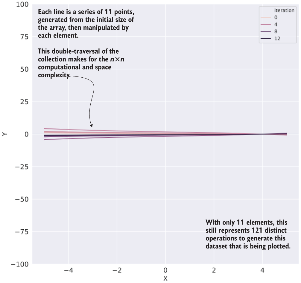
Figure A.11 The data generated from our O(n2) algorithm operating on an array of size 11 (execution time: 433 ms, ~26 KB space required)
Figure A.12 shows the progression in complexity from an array size of 201 (top) to a much more extreme size (2,001, at bottom) when run through this algorithm.

Figure A.12 Comparison of array sizes 201 (time: 8.58 s, space: ~5.82 MB) and 2,001 (time: 1,367 s, space: ~576.57 MB).
As you can see (keep in mind that these plots are generating a series that is plotted for each index position of the input array), a seemingly innocuous collection size can become very large, very quickly, when run through such an algorithm. It’s not too much of a stretch to imagine how much this will affect the runtime performance of a project if code is written with this level of complexity.
A.3 Analyzing decision-tree complexity
Let’s imagine that we’re in the process of building a solution to a problem that, as a core requirement, needs a highly interpretable model structure as its output. Because of this requirement, we choose to use a decision-tree regressor to build a predictive solution.
Since we’re a company that is dedicated to our customers (dogs) and their pets (humans), we need a way to translate our model results into direct and actionable results that can be quickly understood and applied. We’re not looking for a black-box prediction; rather, we’re looking to understand the nature of the correlations in our data and see how the predictions are influenced by the complex system of our features.
After feature engineering is complete and the prototype has been built, we’re in the process of exploring our hyperparameter space in order to hone the automated tuning space for the MVP. After starting the run (with tens of thousands of tuning experiments), we notice that the training of different hyperparameters results in different completion times. In fact, depending on the tested hyperparameters, each test’s runtime can be off by more than an order of magnitude from another. Why?
To explore this concept, let’s step through how a decision-tree regressor works (in the sense of complexity) and evaluate how changing a few hyperparameter settings can affect the runtime. Figure A.13 shows a rather high-level view of what is happening in the algorithm when it is fit upon training data.
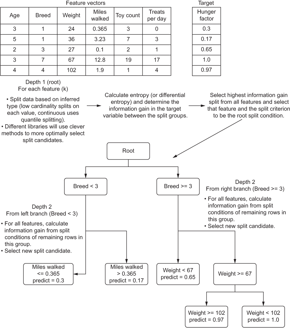
Figure A.13 A high-level explanation of a decision tree algorithm
This diagram is likely familiar to you. The basic structure, functionality, and behavior of the algorithm is covered in great detail in blog posts, other books, and as a foundational concept in learning the basics of ML. What is of interest to our discussion is what affects the computational and space complexity while training the model.
NOTE Figure A.13 is an example only. This model is incredibly overfit and would likely do very poorly against a validation split. With a more realistic data-split volume and a depth restriction, the predictions would be the average of split-branch membership.
To start, we can see that the initial split at the root of the tree requires a determination of which feature to choose to split on first. A scalability factor exists right out of the gate with this algorithm. To determine where to split, we need to measure each feature, split it based on the criterion that the library’s implementation chooses, and calculate the information gain between those splits.
For the purposes of computational complexity, we will refer to the number of features as k. Another component to the calculation of information gain involves the estimation of entropy, based on the size of the dataset being trained upon. This is the n in traditional non-ML complexity. To add to this complexity, we have to traverse each level of the tree. Once a split is realized as the best path, we have to continue to iterate on the features present in the subset of the data, repeatedly, until we hit the criteria set in the hyperparameter that equates to the minimum number of elements to populate a leaf (prediction) node.
Iterating through these nodes represents a computational complexity of O(nlog(n)), as the splits are restricted in size as we move closer to leaf nodes. However, because we are forced to iterate through all features at each of the adjudication nodes, our final computational complexity becomes more akin to O(k × n× log(n)).
We can directly affect the real-world behavior of this worst-case runtime performance by adjusting hyperparameters (remember that O() notation is the worst-case). Of particular note is that some of the hyperparameters can be beneficial to computational complexity and model efficacy (minimum count to create a leaf, maximum depth of tree), while others are negatively correlated (learning rate in other algorithms that utilize stochastic gradient descent, or SGD, for instance).
To illustrate the relationship between a hyperparameter and the runtime performance of a model, let’s look at modifying the maximum depth of a tree in listing A.7. For this example, we’re going to use a freely available open source dataset to illustrate the effect of hyperparameter values that directly influence computational and space complexity of a model. (My apologies for not collecting a dataset regarding dog characteristics and general hunger levels. If anyone wants to create that dataset and release it for common use, please let me know.)
NOTE In listing A.7, in order to demonstrate an excessive depth, I break the rules of tree-based models by one-hot-encoding categorical values. Encoding categorical values in this manner risks a very high chance of preferentially splitting only on the Boolean fields, making a dramatically underfit model if the depth is not sufficient to utilize other fields. Validation of the feature set should always be conducted thoroughly when encoding values to determine if they will create a poor model (or a difficult-to-explain model). Look to bucketing, k-leveling, binary encoding, or enforced-order indexing to solve your ordinal or nominal categorical woes.
Listing A.7 Demonstrating the effects of tree depth on runtime performance
from sklearn.model_selection import train_test_split
from sklearn.tree import DecisionTreeRegressor
from sklearn.metrics import mean_squared_error
import requests
URL = 'https://raw.githubusercontent.com/databrickslabs
/automl-toolkit/master/src/test/resources/fire_data.csv'
file_reader = pd.read_csv(URL)                              ❶
encoded = pd.get_dummies(file_reader,
columns=['month', 'day'])                                   ❷
target_encoded = encoded['burnArea']
features_encoded = encoded.drop('burnArea', axis=1)
x_encoded, X_encoded, y_encoded, Y_encoded = train_test_split(features_encoded,
target_encoded, test_size=0.25)                             ❸
shallow_encoded = DecisionTreeRegressor(max_depth=3,
  min_samples_leaf=3,
  max_features='auto',
  random_state=42)
%timeit -n 500 -r 5 shallow_encoded.fit(x_encoded, y_encoded)
>> 3.22 ms ± 73.7 µs per loop (mean ± std. dev. of 5
runs, 500 loops each)                                       ❹
mid_encoded = DecisionTreeRegressor(max_depth=5,
  min_samples_leaf=3, max_features='auto',
  random_state=42)
%timeit -n 500 -r 5 mid_encoded.fit(x_encoded, y_encoded)
>> 3.79 ms ± 72.8 µs per loop (mean ± std. dev. of 5
runs, 500 loops each)                                       ❺
deep_encoded = DecisionTreeRegressor(max_depth=30,
  min_samples_leaf=1,
  max_features='auto',
  random_state=42)
%timeit -n 500 -r 5 deep_encoded.fit(x_encoded, y_encoded)
>> 5.42 ms ± 143 µs per loop (mean ± std. dev. of 5
runs, 500 loops each)                                       ❻
❶ Pulls in an open source dataset to test against
❷ One-hot-encodes the month and day columns to ensure that we have sufficient features to achieve the necessary depth for this exercise. (See note preceding this listing.)
❸ Gets the train and test split data
❹ A shallow depth of 3 (potentially underfit) reduces the runtime to a minimum baseline.
❺ Moving from a depth of 3 to 5 increases runtime by 17% (some branches will have terminated, limiting the additional time).
❻ Moving to a depth of 30 (actual realized depth of 21 based on this dataset) and reducing the minimum leaf size to 1 captures the worst possible runtime complexity.
As you can see in the timed results of manipulating the hyperparameters, a seemingly insignificant relationship exists between the depth of the tree and the runtime. When we think about this as a percentage change, though, we can start to understand how this could be problematic.
To illustrate the complexity of this tree-based approach, figure A.14 shows the steps that are being taken at each candidate split as the tree is being produced.
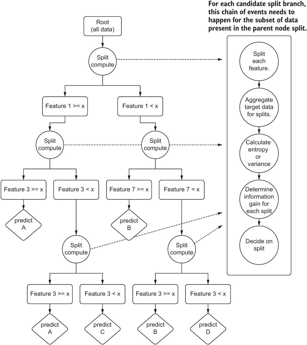
Figure A.14 The computational complexity of a decision tree
Not only do multiple tasks need to be accomplished in order to decide where to split and what to split on, but this entire block of tasks shown on the right side of figure A.14 needs to be completed for each feature on the subset of data that fulfills the prior split conditions at each candidate node. With a tree depth of 30, 40, or 50, we can imagine that this tree becomes quite large rather fast. The runtime will increase comparatively as well.
What happens when the dataset is not, as in this toy example, 517 rows? What happens when we’re training on 500 million rows of data? Setting aside the model performance implications (generalization capabilities) of running to too deep of a tree, when we think about a 68% increase in runtime from a single hyperparameter, the differences in training time can be extremely significant (and costly) if we’re not careful about how we’re controlling the hyperparameters of the model.
Now that you’ve seen how computationally expensive hyperparameter tuning is, in the next section we’ll look at the computational and space complexities of different model families.
A.4 General algorithmic complexity for ML
While we won’t be talking about the implementation details of any other ML algorithm (as I’ve mentioned before, there are books devoted to that subject), we can look at one further example. Let’s suppose we are dealing with an incredibly large dataset. It has 10 million rows of training data, 1 million rows of test data, and a feature set of 15 elements.
With a dataset this big, we’re obviously going to be using distributed ML with the SparkML packages. After doing some initial testing on the 15 features within the vector, a decision is made to start improving the performance to try to get better error-metric performance. Since we’re using a generalized linear model for the project, we’re handling collinearity checks on all features and are scaling the features appropriately.
For this work, we split the team into two groups. Group 1 works on adding a single validated feature at a time, checking the improvement or degradation of the prediction performance against the test set at each iteration. While this is slow going, group 1 is able to cull or add potential candidates one at a time and have a relatively predictable runtime performance from run to run.
The members of group 2, on the other hand, add 100 potential features that they think will make the model better. They execute the training run and wait. They go to lunch, have a delightful conversation, and return back to the office. Six hours later, the Spark cluster is still running with all executors pegged at >90% CPU. It continues to run overnight as well.
The main problem here is the increase in computational complexity. While the n of the model hasn’t changed at all (training data is still the exact same size), the reason for the longer runtime is simply the increased feature size. For large datasets, this becomes a bit of a problem because of the way that the optimizer functions.
While traditional linear solvers (ordinary least squares, for instance) can rely on solving a best fit through a closed-form solution involving matrix inversion, on large datasets that need to be distributed, this isn’t an option. Other solvers have to be employed for optimizing in a distributed system. Since we’re using a distributed system, we’re looking at SGD. Being an iterative process, SGD will perform optimization by taking steps along a local gradient of the tuning history.
To get a simplified sense of how SGD works, see figure A.15. This 3D plot represents a walk of the solver along a series of gradients in its attempt to find the global minima error for a particular set of coefficients for the linear equation being generated.
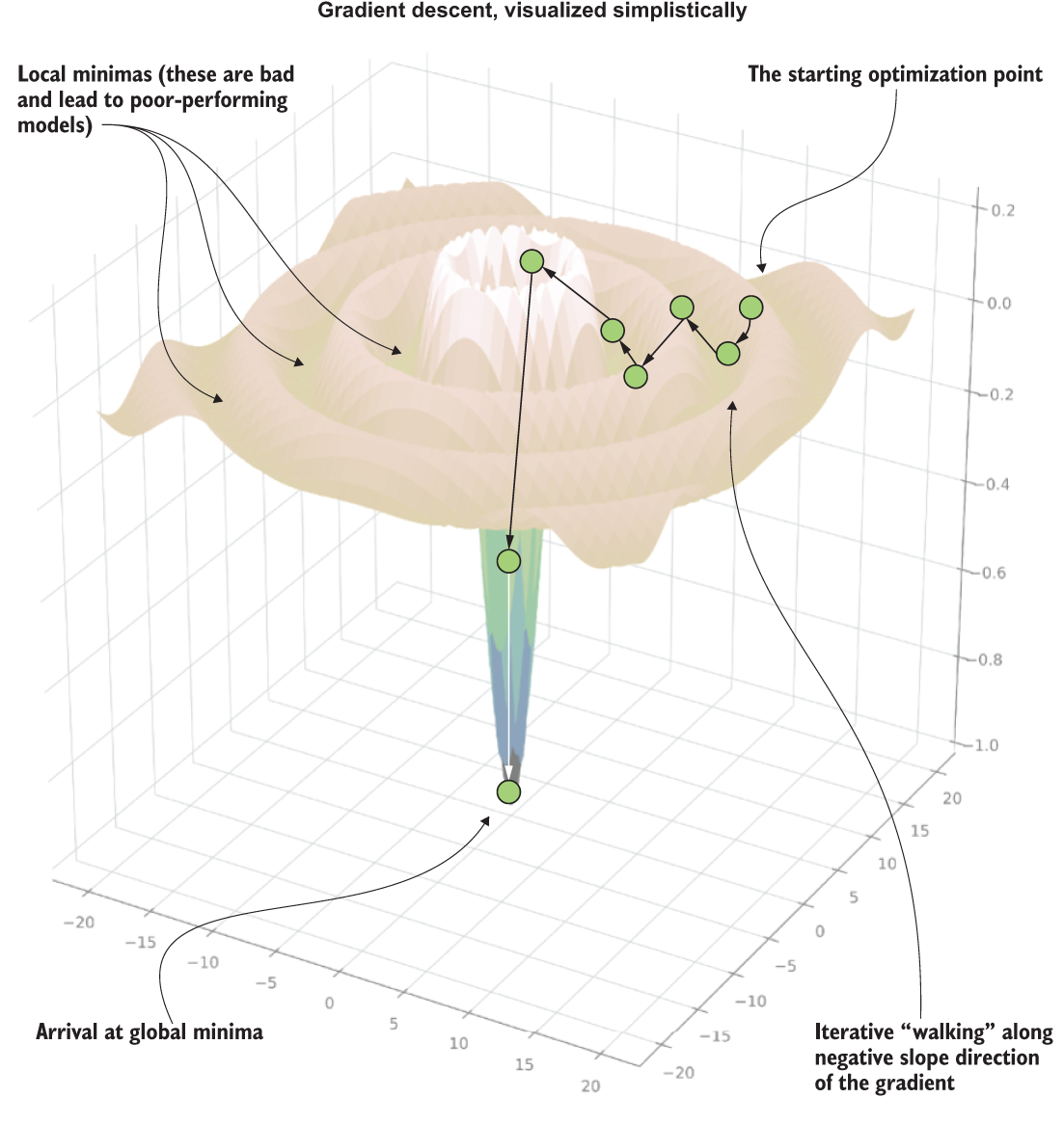
Figure A.15 A visual representation (with artistic liberties) of the SGD process of searching for minimization during optimization
Note Stochastic gradient descent will proceed along fixed-distance adjustments to attempt to arrive at the best fit to the test data (error minimization). It will stop when either the descent flattens to a slope of 0 and subsequent iterations within a threshold show no improvement or maximum iterations is reached.
Notice the iterative search that is occurring. This series of attempts to get the best fit of the equation to the target variable involves making adjustments to each of the coefficients for each element of the feature vector. Naturally, as the size of the vector increases, the number of coefficient evaluations grows. This process needs to occur for each iterative walk that is occurring.
However, a bit of a wrench is being thrown into this situation. SGD and iterative methodologies of its ilk (such as genetic algorithms) don’t have a simple solution for determining computational complexity.
The reason for this (which is also true for other comparable iterating solvers, like limited memory Broyden-Fletcher-Goldfarb-Shanno, or L-BFGS) is that the nature of the optimization minima in both a local and global sense is highly dependent on the composition of the feature data (distributions and inferred structural types), the nature of the target, and the complexity of the feature space (feature count).
These algorithms all have settings for maximum number of iterations to achieve a best-effort optimization to a global minima state, but there is no guarantee that optimization will happen before hitting that iterator maximum count. Conversely, one of the challenges that can arise when determining how long training is going to take revolves around the complexity of optimization. If SGD (or other iterative optimizers) can arrive at a (hopefully, global) minima in a relatively short number of iterations, training will terminate long before the maximum iteration count is reached.
Because of these considerations, table A.2 is a rough estimate of theoretical worst-case computational complexity in common traditional ML algorithms.
Table A.2 Estimation of computational complexity for different model families
The most common aspect of all of these complexities involves separate factors: the number of vectors used for training (row count in a DataFrame) and the number of features in the vector. An increase in the count of either of these has a direct effect on the runtime performance. Many ML algorithms have an exponential relationship between computational time and the size of the input feature vector. Setting aside the intricacies of different optimization methodologies, the solver of a given algorithm can have its performance impacted adversely as a feature set size grows. While each algorithm family has its own nuanced relationships to both feature size and training sample sizes, understanding the impact that feature counts have in general is an important concept to remember while in the early stages of a project's development.
As we saw in the previous section, the depth of a decision tree can influence the runtime performance, since it is searching through more splits, and thus taking more time to do so. Nearly all models have parameters that give flexibility to the application’s practitioner that will directly influence the predictive power of a model (typically at the expense of runtime and memory pressure).
In general, it’s a good idea to become familiar with the computational and space complexities of ML models. Knowing the impact to the business of selecting one type of model over another (provided that they’re capable of solving the problem in a similar manner) can make a difference of orders of magnitude in cost after everything is in production. I’ve personally made the decision many times to use something that was slightly worse in predictive capabilities because it could run in a fraction of the time of an alternative that was many times more expensive to execute.
Remember, at the end of the day, we’re here to solve problems for the business. Getting a 1% increase in prediction accuracy at the expense of 50 times the cost creates a new type of problem for the business while solving what you set out to do.