16 Production infrastructure

This chapter covers

• Implementing passive retraining with the use of a model registry
• Utilizing a feature store for model training and inference
• Selecting an appropriate serving architecture for ML solutions

Utilizing ML in a real-world use case to solve a complex problem is challenging. The sheer number of skills needed to take a company’s data (frequently messy, partially complete, and rife with quality issues), select an appropriate algorithm, tune a pipeline, and validate that the prediction output of a model (or an ensemble of models) solves the problem to the satisfaction of the business is daunting. The complexity of an ML-backed project does not end with the creation of an acceptably performing model, though. The architectural considerations and implementation details can add significant challenges to a project if they aren’t made correctly.

Every day there seems to be a new open sourced tech stack that promises an easier deployment strategy or a magical automated solution that meets the needs of all. With this constant deluge of tools and platforms, making a decision on where to go to meet the needs of a particular project can be intimidating.

A cursory glance at the offerings available may seem to indicate that the most logical plan is to stick to a single paradigm for everything (for example, deploy every model as a REST API service). Keeping every ML project aligned in a common architecture and implementation certainly simplifies the release deployment. However, nothing could be further from the truth. Just as when selecting algorithms, there’s no “one size fits all” for production infrastructure.

The goal of this chapter is to introduce common generic themes and solutions that can be applied to model prediction architecture. After covering the basic tooling that obfuscates the complexity and minutiae of production ML services, we will delve into generic architectures that can be employed to meet the needs of different projects.

The goal in any serving architecture is to build the minimally featured, least complex, and cheapest solution that still meets the needs of consuming the model’s output. With consistency and efficiency in serving (SLA and prediction-volume considerations) as the primary focus for production work, there are several key concepts and methodologies to be aware of to make this last-mile aspect of ML project work as painless as possible.

16.1 Artifact management

Let’s imagine that we’re still working at the fire-risk department of the forest service introduced in chapter 15. In our efforts to effectively dispatch personnel and equipment to high-risk areas in the park system, we’ve arrived at a solution that works remarkably well. Our features are locked in and are stable over time. We’ve evaluated the performance of the predictions and are seeing genuine value from the model.

Throughout this process of getting the features into a good state, we’ve been iterating through the improvement cycle, shown in figure 16.1.

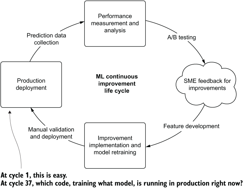
Figure 16.1 Improvements to a deployed model on the road to production steady-state operation

As this cycle shows, we’ve been iteratively releasing new versions of the model, testing against a baseline deployment, collecting feedback, and working to improve the predictions. At some point, however, we’ll be going into model-sustaining mode.

We’ve worked as hard as we can to improve the features going into the model and have found that the return on investment (ROI) of continuing to add new data elements to the project is simply not worth it. We’re now in the position of scheduled passive retraining of our model based on new data coming in over time.

When we’re at this steady-state point, the last thing that we want to do is to have one of the DS team members spend an afternoon manually retraining a model, manually comparing its results to the current production-deployed model with ad hoc analysis, and deciding on whether the model should be updated.

The measurement, adjudication, and decision on whether to replace the model with a newly retrained one can be automated with a passive retraining system. Figure 16.2 shows this concept of a scheduled retraining event.

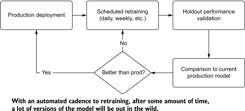
Figure 16.2 Logical diagram of a passive retraining system

With this automation of scheduled retraining in place, the primary concern with this system is knowing what is running in production. For instance, what happens if a problem is uncovered in production after a new version is released? What can we do to recover from a concept drift that has dramatically affected a retraining event? How do we roll back the model to the previous version without having to rebuild it? We can allay these concerns by using a model registry.

16.1.1 MLflow’s model registry

In this situation that we find ourselves in, with scheduled updates to a model happening autonomously, it is important for us to know the state of production deployment. Not only do we need to know the current state, but if questions arise about performance of a passive retraining system in the past, we need to have a means of investigating the historical provenance of the model. Figure 16.3 compares using and not using a registry for tracking provenance in order to explain a historical issue.

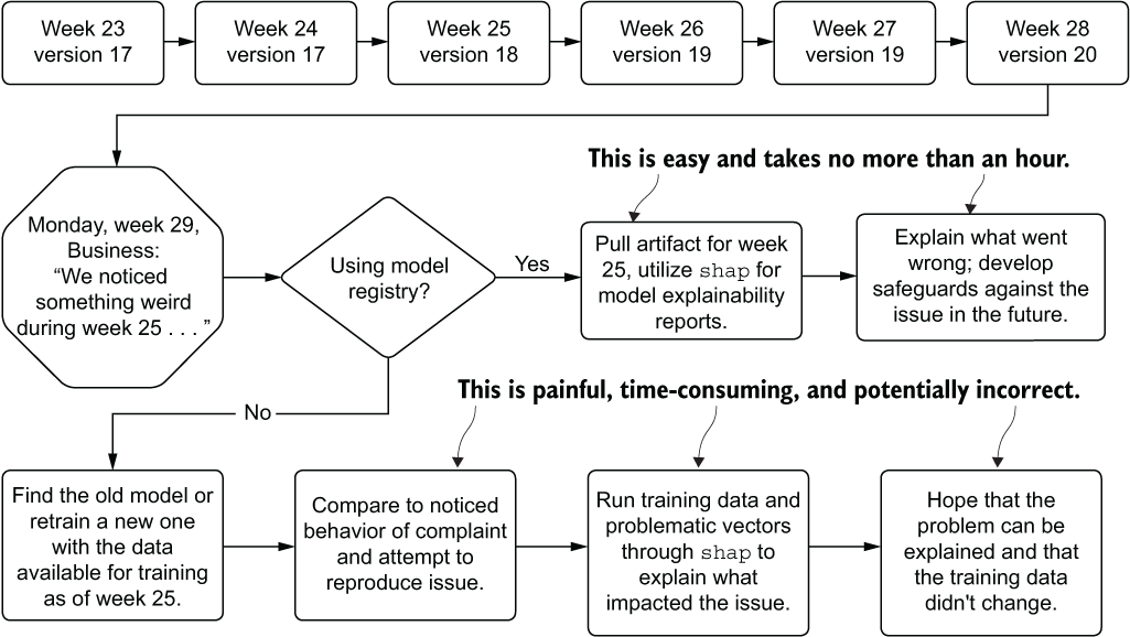
Figure 16.3 Passive retraining schedule with a historic issue found far in the future

As you can see, the process for attempting to re-create a past run is fraught with peril; we have a high risk of being unable to reproduce the issue that the business found in historical predictions. With no registry to record the artifacts utilized in production, manual work must be done to re-create the model’s original conditions. This can be incredible challenging (if not impossible) in most companies because changes may have occurred to the underlying data used to train the model, rendering it impossible to re-create that state.

The preferred approach, as shown in figure 16.3, is to utilize a model registry service. MLflow, for instance, offers exactly this functionality within its APIs, allowing us to log details of each retraining run to the tracking server, handle production promotion if the scheduled retraining job performs better on holdout data, and archive the older model for future reference. If we had used this framework, the process of testing conditions of a model that had at one point run in production would be as simple as recalling the artifact from the registry entry, loading it into a notebook environment, and generating the explainable correlation reports with tools such as shap.

16.1.2 Interfacing with the model registry

To get a feel for how this code would look to support an integration with the model registry service of MLflow, let’s adapt our use case to support this passive retraining functionality. To start, we need to create an adjudication system that checks the current production model’s performance against the scheduled retraining results. After building that comparison, we can interface with the registry service to replace the current production model with the newer model (if it’s better), or stay with the current production model based on its performance against the same holdout data that the new model was tested against.

Let’s look at an example of how to interface with the MLflow model registry to support automated passive retraining that retains provenance of the model’s state over time. Listing 16.1 establishes the first portion of what we need to build to have a historical status table of each scheduled retraining event.

NOTE To see all of the import statements and the full example that integrates with these snippets, see the companion notebook to this chapter in the GitHub repository for this book at https://github.com/BenWilson2/ML-Engineering.

Listing 16.1 Registry state row generation and logging

@dataclass
class Registry:                                             ❶
  model_name: str
  production_version: int
  updated: bool
  training_time: str
class RegistryStructure:                                    ❷
  def __init__(self, data):
    self.data = data
  def generate_row(self):
    spark_df = spark.createDataFrame(pd.DataFrame(
      [vars(self.data)]))                                   ❸
    return (spark_df.withColumn("training_time", 
F.to_timestamp(F.col("training_time")))
            .withColumn("production_version", 
F.col("production_version").cast("long")))
class RegistryLogging:
  def __init__(self, 
               database, 
               table, 
               delta_location, 
               model_name, 
               production_version, 
               updated):
    self.database = database
    self.table = table
    self.delta_location = delta_location
    self.entry_data = Registry(model_name, 
                               production_version, 
                               updated, 
                               self._get_time())           ❹
  @classmethod
  def _get_time(self):
    return datetime.today().strftime('%Y-%m-%d %H:%M:%S')
  def _check_exists(self):                                 ❺
    return spark._jsparkSession.catalog().tableExists(
      self.database, self.table)
  def write_entry(self):                                   ❻
    log_row = RegistryStructure(self.entry_data).generate_row()
    log_row.write.format("delta").mode("append").save(self.delta_location)
    if not self._check_exists():
      spark.sql(f"""CREATE TABLE IF NOT EXISTS 
         {self.database}.{self.table} 
         USING DELTA LOCATION 
         '{self.delta_location}';""")

❶ A data class to wrap the data we’re going to be logging

❷ Class for converting the registration data to a Spark DataFrame to write a row to a delta table for provenance

❸ Accesses the members of the data class in a shorthand fashion to cast to a pandas DataFrame and then a Spark DataFrame (leveraging implicit type inferences)

❹ Builds the Spark DataFrame row at class initialization

❺ Method for determining if the delta table has been created yet

❻ Writes the log data to Delta in append mode and creates the table reference in the Hive Metastore if it doesn’t already exist

This code helps set the stage for the provenance of the model-training history. Since we’re looking to automate the retraining on a schedule, it’s far easier to have a tracking table that refers to the history of changes in a centralized location. If we have multiple builds of this model, as well as other projects that are registered, we can have a single snapshot view of the state of production passive retraining without needing to do anything more than write a simple query.

Listing 16.2 illustrates what a query of this table would look like. With multiple models logged to a transaction history table like this, adding df.filter(F.col("model_ name"=="<projecttitle>") allows for rapid access to the historical log for a single model.

Listing 16.2 Querying the registry state table

from pyspark.sql import functions as F
REGISTRY_TABLE = "mleng_demo.registry_status"
display(spark.table(REGISTRY_TABLE).orderBy(F.col("training_time"))    ❶

❶ Since we’ve registered the table in our row-input stage earlier, we can refer to it directly by <database>.<table_name> reference. We can then order the commits chronologically.

Executing this code results in figure 16.4. In addition to this log, the model registry within MLflow also has a GUI. Figure 16.5 shows a screen capture of the GUI that matches to the registry table from listing 16.2.

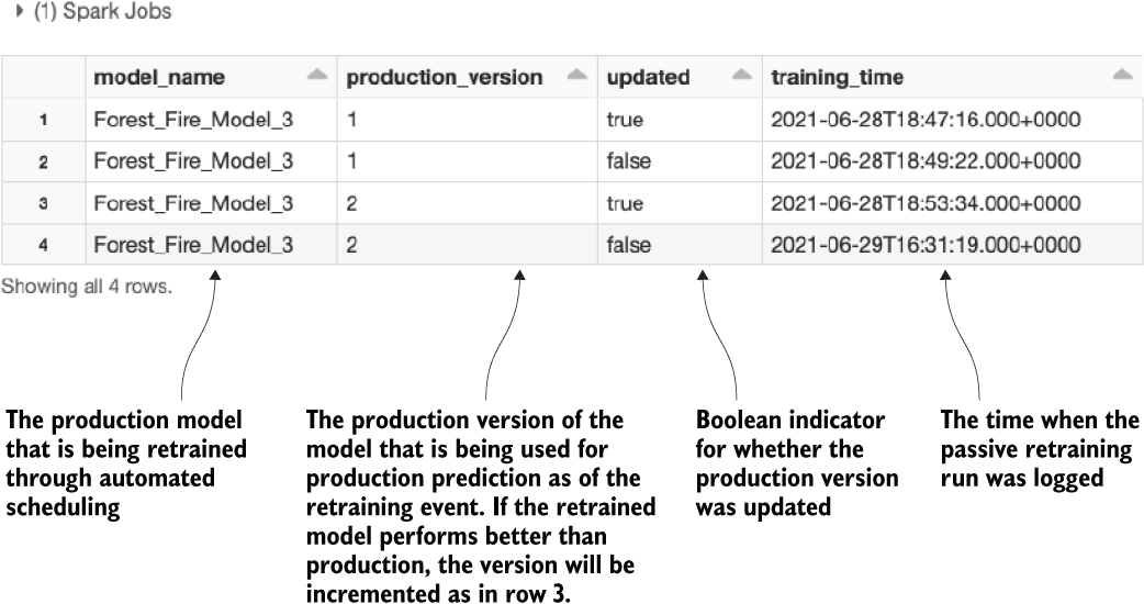
Figure 16.4 Querying the registry state transaction table

Now that we’ve set up the historical tracking functionality, we can write the interface to MLflow’s registry server to support passive retraining. Listing 16.3 shows the implementation for leveraging the tracking server’s entries, the registry service for querying current production metadata, and an automated state transition of the retrained model for supplanting the current production model if it performs better.

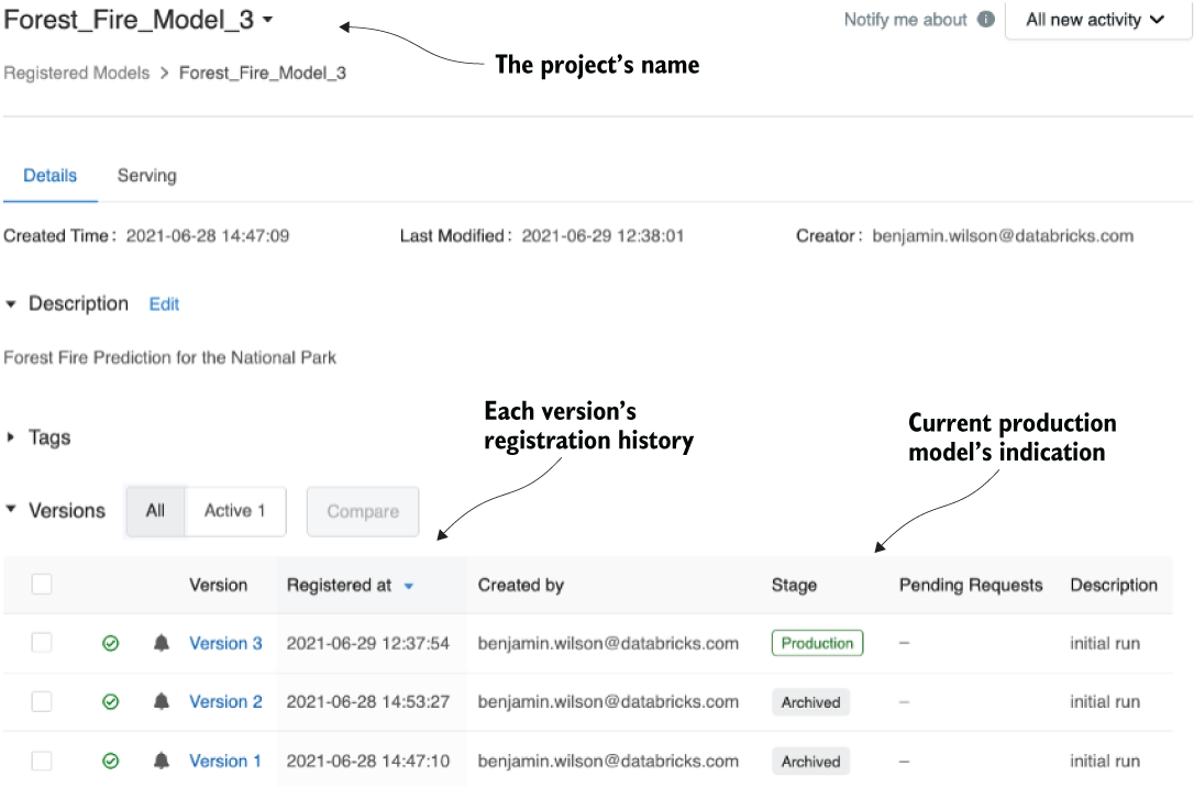
Figure 16.5 The MLflow model registry GUI for our experiments

Listing 16.3 Passive retraining model registration logic

class ModelRegistration:
  def __init__(self, experiment_name, experiment_title, model_name, metric,
               direction):
    self.experiment_name = experiment_name
    self.experiment_title = experiment_title
    self.model_name = model_name
    self.metric = metric
    self.direction = direction
    self.client = MlflowClient()
    self.experiment_id = mlflow.get_experiment_by_name(experiment_name).experiment_id
  def _get_best_run_info(self, key):                                        ❶
    run_data = mlflow.search_runs(
      self.experiment_id, 
      order_by=[f"metrics.{self.metric} {self.direction}"])
    return run_data.head(1)[key].values[0]
  def _get_registered_status(self):
    return self.client.get_registered_model(name=self.experiment_title)
  def _get_current_prod(self):                                              ❷
    return ([x.run_id for x in self._get_registered_status().latest_versions
     if x.current_stage == "Production"][0])
  def _get_prod_version(self):
    return int([x.version for x in 
     self._get_registered_status().latest_versions
             if x.current_stage == "Production"][0])
  def _get_metric(self, run_id):
    return mlflow.get_run(run_id).data.metrics.get(self.metric)
  def _find_best(self):                                                     ❸
    try: 
      current_prod_id = self._get_current_prod()
      prod_metric = self._get_metric(current_prod_id)
    except mlflow.exceptions.RestException:
      current_prod_id = -1
      prod_metric = 1e7
    best_id = self._get_best_run_info('run_id')
    best_metric = self._get_metric(best_id)
    if self.direction == "ASC":
      if prod_metric < best_metric:
        return current_prod_id
      else:
        return best_id
    else:
      if prod_metric > best_metric:
        return current_prod_id
      else:
        return best_id
  def _generate_artifact_path(self, run_id):
    return f"runs:/{run_id}/{self.model_name}"
  def register_best(self, registration_message, logging_location, log_db,
                    log_table):                                             ❹
    best_id = self._find_best()
    try:
      current_prod = self._get_current_prod()
      current_prod_version = self._get_prod_version()
    except mlflow.exceptions.RestException:
      current_prod = -1
      current_prod_version = -1
    updated = current_prod != best_id
    if updated:
      register_new = mlflow.register_model(self._generate_artifact_path(best_id),
                                   self.experiment_title)
      self.client.update_registered_model(name=register_new.name, 
                                          description="Forest Fire 
                                          Prediction for the National Park")
      self.client.update_model_version(name=register_new.name, 
                                       version=register_new.version, 
                                       description=registration_message)
      self.client.transition_model_version_stage(name=register_new.name, 
                                                 version=register_new.version,
                                                 stage="Production")
      if current_prod_version > 0:
        self.client.transition_model_version_stage(
          name=register_new.name, 
          version=current_prod_version,
         stage="Archived")
      RegistryLogging(log_db, 
            log_table, 
            logging_location, 
            self.experiment_title,  
            int(register_new.version), 
            updated).write_entry()
      return "upgraded prod"
    else:
      RegistryLogging(log_db, 
            log_table, 
            logging_location, 
            self.experiment_title, 
            int(current_prod_version), 
            updated).write_entry()
      return "no change"
  def get_model_as_udf(self):                                               ❺
    prod_id = self._get_current_prod()
    artifact_uri = self._generate_artifact_path(prod_id)
    return mlflow.pyfunc.spark_udf(spark, model_uri=artifact_uri)

❶ Extracts all the previous run data for the history of the production deployment and returns the run ID that has the best performance against the validation data

❷ Query for the model currently registered as “production deployed’ in the registry

❸ Method for determining if the current scheduled passive retraining run is performing better than production on its holdout data. It will return the run_id of the best logged run.

❹ Utilizes the MLflow Model Registry API to register the new model if it is better, and de-registers the current production model if it’s being replaced

❺ Acquires the current production model for batch inference on a Spark DataFrame using a Python UDF

This code allows us to fully manage the passive retraining of this model implementation (see the companion GitHub repository for this book for the full code). By leveraging the MLflow Model Registry API, we can meet the needs of production-scheduled predictions through having a one-line access to the model artifact.

This greatly simplifies the prediction batch-scheduled job, but also meets the needs of the investigation we began discussing in this section. Having the ability to retrieve the model with such ease, we can manually test the feature data against that model, run simulations with the use of tools like shap, and rapidly answer business questions without having to struggle with re-creating a potentially impossible state.

In the same vein of using a model registry to keep track of the model artifacts, the features being used to train models and predict with the use of models can be catalogued for efficiency’s sake as well. This concept is realized through feature stores.

16.2 Feature stores

We briefly touched on using a feature store in the preceding chapter. While it is important to understand the justification for and benefits of implementing a feature store (namely, that of consistency, reusability, and testability), seeing an application of a relatively nascent technology is more relevant than discussing the theory. Here, we’re going to look at a scenario that I struggled through, involving the importance of utilizing a feature store to enforce consistency throughout an organization leveraging both ML and advanced analytics.

Let’s imagine that we work at a company that has multiple DS teams. Within the engineering group, the main DS team focuses on company-wide initiatives. This team works mostly on large-scale projects involving critical services that can be employed by any group within the company, as well as customer-facing services. Spread among departments are a smattering of independent contributor DS employees who have been hired by and report to their respective department heads. While collaboration occurs, the main datasets used by the core DS team are not open for the independent DS employees’ use.

At the start of a new year, a department head hires a new DS straight out of a university program. Well-intentioned, driven, and passionate, this new hire immediately gets to work on the initiatives that this department head wants investigated. In the process of analyzing the characteristics of the customers of the company, the new hire come across a production table that contains probabilities for customers to make a call-center complaint. Curious, the new DS begins analyzing the predictions against the data that is in the data warehouse for their department.

Unable to reconcile any feature data to the predictions, the DS begins working on a new model prototype to try to improve upon the complaint prediction solution. After spending a few weeks, the DS presents their findings to their department head. Given the go-ahead to work on this project, the DS proceeds to build a project in their analytics department workspace. After several months, the DS presents their findings at a company all-hands meeting.

Confused, the core DS team asks why this project is being worked on and for further details on the implementation. In less than an hour, the core DS team is able to explain why the independent DS’s solution worked so well: they leaked the label. Figure 16.6 illustrates the core DS team’s explanation: the data required to build any new model or perform extensive analysis of the data collected from users is walled off by the silo surrounding the core DS team’s engineering department.

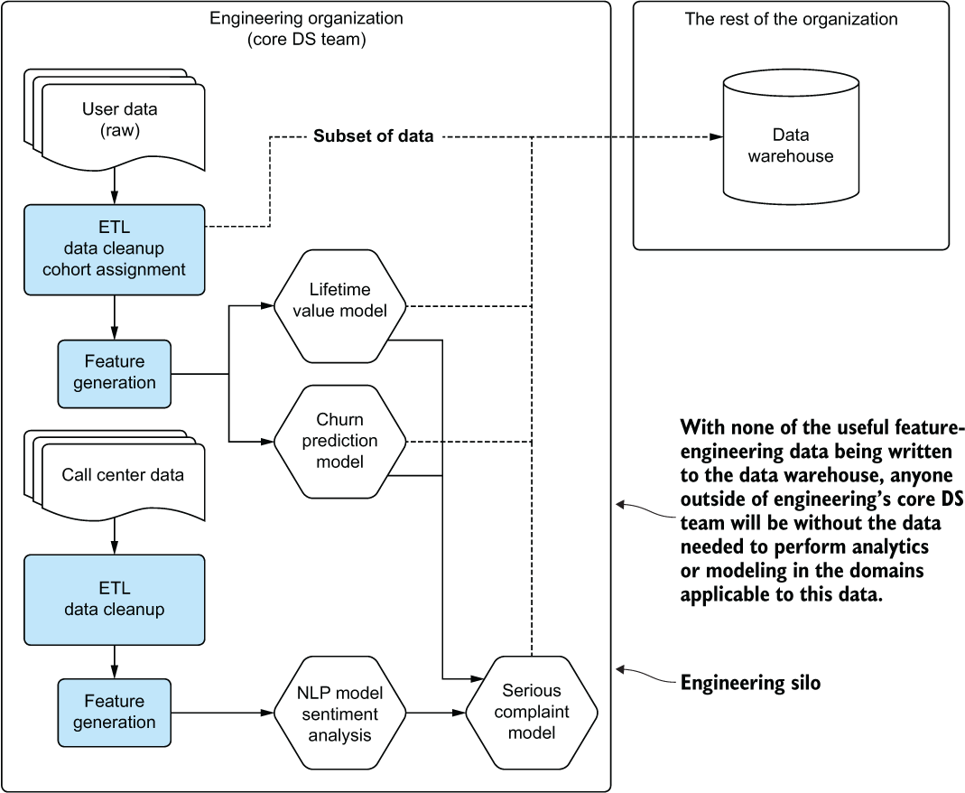
Figure 16.6 The engineering silo that keeps raw data and calculated features away from the rest of the organization

The data being used for training that was present in the department’s data warehouse was being fed from the core DS team’s production solution. Each source feature used to train the core model was inaccessible to anyone apart from engineering and production processes.

While this scenario is extreme, it did, in fact, happen. The core team could have helped to avoid this by providing an accessible source for the generated feature data, opening the access to allow other teams to utilize these highly curated data points for additional projects. By registering their data with appropriate labels and documentation, they could have saved this poor DS a lot of effort.

16.2.1 What a feature store is used for

Solving the data silo issue in our scenario is among the most compelling reasons to use a feature store. When dealing with a distributed DS capability throughout an organization, the benefits of standardization and accessibility are seen through a reduction in redundant work, incongruous analyses, and general confusion surrounding the veracity of solutions.

However, having a feature store enables an organization to do far more with its data than just quality-control it. To illustrate these benefits, figure 16.7 shows a high-level code architecture for model building and serving with and without a feature store.

The top portion of figure 16.7 shows the historical reality of ML development for projects. Tightly coupled feature-engineering code is developed inline to the model tuning and training code to generate models that are more effective than they would be if trained on the raw data. While this architecture makes sense from a development perspective of generating a good model, it creates an issue when developing the prediction code base (as shown at the top right of figure 16.7).

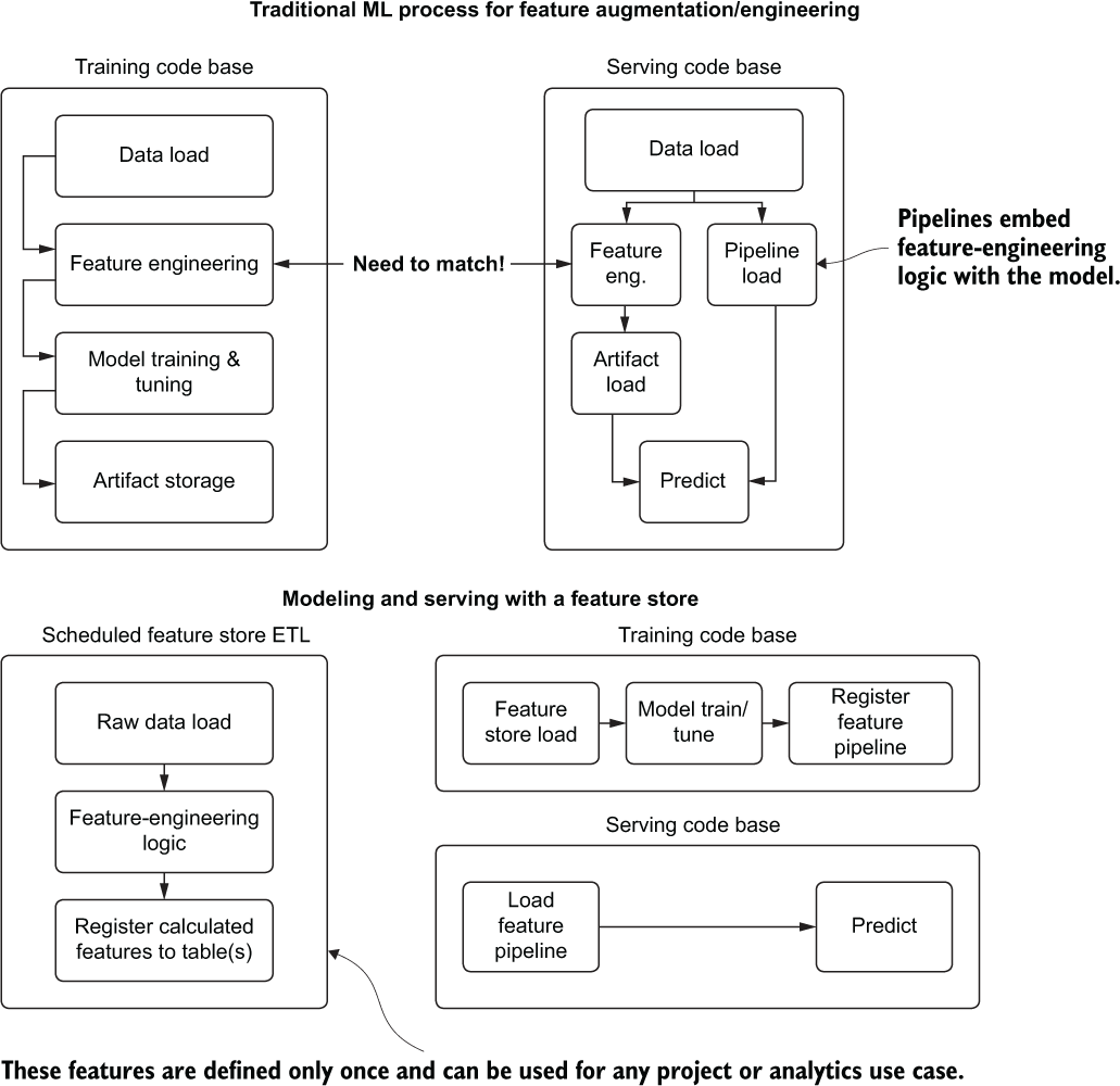
Figure 16.7 Comparison of using a feature store versus not using one for ML development

Any operations that are done to the raw data now need to be ported over to this serving code, presenting an opportunity for errors and inconsistencies in the model vector. Alternatives to this approach can help eliminate the chances of data inconsistency, however:

• Use a pipeline (most major ML frameworks have them).
• Abstract feature-engineering code into a package that training and serving can both call.
• Write traditional ETL to generate features and store them.

Each of these approaches has its own downsides, though. Pipelines are great and should be used, but they entangle useful feature-engineering logic with a particular model’s implementation, isolating it from being utilized elsewhere. There’s simply no easy way to reuse the features for other projects (not to mention it’s nearly impossible for an analyst to decouple the feature-engineering stages from an ML pipeline without help).

Abstracting feature-engineering code certainly helps with code reusability and solves the consistency problem for the projects requiring the use of those features. But access to these features outside the DS team is still walled off. The other downside is that it’s another code base that needs to be maintained, tested, and frequently updated.

Let’s look at an example of interacting with a feature store, using the Databricks implementation to see the benefits in action.

NOTE Implementations of features of this nature that are built by a company are subject to change. APIs, feature details, and associated functionality may change, sometimes quite significantly, over time. This example of one such implementation of a feature store is presented for demonstration purposes.

16.2.2 Using a feature store

The first step in utilizing a feature store is to define a DataFrame representation of the processing involved in creating the features we’d like to use for modeling and analytics. The following listing shows a list of functions that are acting on a raw dataset to generate new features.

Listing 16.4 Feature-engineering logic

from dataclasses import dataclass
from typing import List
from pyspark.sql.types import *
from pyspark.sql import functions as F
from pyspark.sql.functions import when
@dataclass
class SchemaTypes:
  string_cols: List[str]
  non_string_cols: List[str]
def get_col_types(df):
  schema = df.schema
  strings = [x.name for x in schema if x.dataType == StringType()]
  non_strings = [x for x in schema.names if x not in strings]
  return SchemaTypes(strings, non_strings)
def clean_messy_strings(df):                                 ❶
  cols = get_col_types(df)
  return df.select(*cols.non_string_cols, *[F.regexp_replace(F.col(x), " ", 
    "").alias(x) for x in cols.string_cols])
def fill_missing(df):                                        ❷
  cols = get_col_types(df)
  return df.select(
*cols.non_string_cols, *[when(F.col(x) == "?", 
"Unknown").otherwise(F.col(x)).alias(x) for x in cols.string_cols])
def convert_label(df, label, true_condition_string):         ❸
  return df.withColumn(label, when(F.col(label) == 
true_condition_string,1).otherwise(0))
def generate_features(df, id_augment):                       ❹
  overtime = df.withColumn("overtime", 
when(F.col("hours_worked_per_week") > 40, 1).otherwise(0))
  net_pos = overtime.withColumn("gains", 
when(F.col("capital_gain") > F.col("capital_loss"), 1).otherwise(0))
  high_edu = net_pos.withColumn("highly_educated", 
when(F.col("education_years") >= 16, 2)
.when(F.col("education_years") > 12, 1).otherwise(0))
        gender = high_edu.withColumn("gender_key", 
when(F.col("gender") == "Female", 1).otherwise(0))
  keys = gender.withColumn("id", 
F.monotonically_increasing_id() + F.lit(id_augment))
  return keys
def data_augmentation(df, 
                      label, 
                      label_true_condition, 
                      id_augment=0):                         ❺
  clean_strings = clean_messy_strings(df)
  missing_filled = fill_missing(clean_strings)
  corrected_label = convert_label(missing_filled, 
                                  label, 
                                  label_true_condition)
  additional_features = generate_features(corrected_label, 
                                           id_augment)
  return additional_features

❶ General cleanup to strip out leading whitespaces from the dataset’s string columns

❷ Converts placeholder unknown values to a more useful string

❸ Converts the target from a string to a Boolean binary value

❹ Creates new encoded features for the model

❺ Executes all the feature-engineering stages, returning a Spark DataFrame

Once we execute this code, we’re left with a DataFrame and the requisite embedded logic for creating those additional columns. With this, we can initialize the feature store client and register the table, as shown in the next listing.

Listing 16.5 Register the feature engineering to the feature store

from databricks import feature_store               ❶
fs = feature_store.FeatureStoreClient()            ❷
FEATURE_TABLE = "ds_database.salary_features"      ❸
FEATURE_KEYS = ["id"]                              ❹
FEATURE_PARTITION = "gender"                       ❺
fs.create_feature_table(
  name=FEATURE_TABLE,
  keys=["id"],
  features_df=data_augmentation(raw_data, 
                                "income", 
                                ">50K"),           ❻
  partition_columns=FEATURE_PARTITION,
  description="Adult Salary Data. Raw Features."   ❼
)

❶ The library that contains the APIs to interface with the feature store

❷ Initializes the feature store client to interact with the feature store APIs

❸ The database and table name where this feature table will be registered

❹ A primary key to affect joins

❺ Sets a partition key to make querying perform better if operations utilize that key

❻ Specifies the processing history for the DataFrame that will be used to define the feature store table (from listing 16.4)

❼ Adds a description to let others know this table’s content

After executing the registration of the feature table, we can ensure that it is populated with new data as it comes in through a lightweight scheduled ETL. The following listing shows how simple this is.

Listing 16.6 Feature store ETL update

new_data = spark.table(“prod_db.salary_raw”)             ❶
processed_new_data = data_augmentation(new_data, 
                                        "income", 
                                        ">50K", 
                                        table_counts)    ❷
fs = feature_store.FeatureStoreClient()
fs.write_table(                                          ❸
  name=FEATURE_TABLE,
  df=processed_new_data,
  mode='merge'
)

❶ Reads in new raw data that needs processing through the feature-generation logic

❷ Processes the data through the feature logic

❸ Writes the new feature data through the previously registered feature table in merge mode to append new rows

Now that we’ve registered the table, the real key to its utility is in registering a model using it as input. To start accessing the defined features within a feature table, we need to define lookup accessors to each of the fields. The next listing shows how to do this data acquisition on the fields that we want to utilize for our income prediction model.

Listing 16.7 Feature acquisition for modeling

from databricks.feature_store import FeatureLookup          ❶
def generate_lookup(table, feature, key):
  return FeatureLookup(
    table_name=table,
    feature_name=feature,
    lookup_key=key
  )
features = ["overtime", "gains", "highly_educated", "age",
            "education_years", "hours_worked_per_week", 
            "gender_key"]                                   ❷
lookups = [generate_lookup(FEATURE_TABLE, x, "id") 
            for x in features]                              ❸

❶ The API to interface with the feature store to obtain references for modeling purposes

❷ The list of field names that our model will be using

❸ The lookup objects for each of the features

Now that we’ve defined the lookup references, we can employ them in the training of a simple model, as shown in listing 16.8.

NOTE This is an abbreviated snippet of the full code. Please see the companion code in the book’s repository at https://github.com/BenWilson2/ML-Engineering for the full-length example.

Listing 16.8 Register a model integrated with feature store

import mlflow
from catboost import CatBoostClassifier, metrics as cb_metrics
from sklearn.model_selection import train_test_split
EXPERIMENT_TITLE = "Adult_Catboost"
MODEL_TYPE = "adult_catboost_classifier"
EXPERIMENT_NAME = f"/Users/me/Book/{EXPERIMENT_TITLE}"
mlflow.set_experiment(EXPERIMENT_NAME)
with mlflow.start_run():
  TEST_SIZE = 0.15
  training_df = spark.table(FEATURE_TABLE).select("id", "income")
  training_data = fs.create_training_set(
    df=training_df,
    feature_lookups=lookups,
    label="income",
    exclude_columns=['id', 'final_weight', 'capital_gain', 'capital_loss']) ❶
  train_df = training_data.load_df().toPandas()                             ❷
  X = train_df.drop(['income'], axis=1)
  y = train_df.income
  X_train, X_test, y_train, y_test = train_test_split(X, y, test_size=TEST_SIZE,
                                                      random_state=42,
                                                      stratify=y)
  model = CatBoostClassifier(iterations=10000, learning_rate=0.00001, 
    custom_loss=[cb_metrics.AUC()]).fit(X_train, y_train, 
      eval_set=(X_test, y_test), logging_level="Verbose")
  fs.log_model(model, MODEL_TYPE, flavor=mlflow.catboost,
    training_set=training_data, registered_model_name=MODEL_TYPE)           ❸

❶ Specifies the fields that will be used for training the model by using the lookups defined in the preceding listing

❷ Converts the Spark DataFrame to a pandas DataFrame to utilize catboost

❸ Registers the model to the feature store API so the feature-engineering tasks will be merged to the model artifact

With this code, we have a data source defined as a linkage to a feature store table, a model utilizing those features for training, and a registration of the artifact dependency chain to the feature store’s integration with MLflow.

The final aspect of a feature store’s attractiveness from a consistency and utility perspective is in the serving of the model. Suppose we want to do a daily batch prediction using this model. If we were to use something other than the feature store approach, we’d have to either reproduce the feature-generation logic or call an external package, processing on the raw data, to get our features. Instead, we must write only a few lines of code to get an output of batch predictions.

Listing 16.9 Run batch predictions with feature store registered model

from mlflow.tracking.client import MlflowClient
client = MlflowClient()
experiment_id = mlflow.get_experiment_by_name(EXPERIMENT_NAME).experiment_id ❶
run_id = mlflow.search_runs(experiment_id, 
    order_by=["start_time DESC"]
   ).head(1)["run_id"].values[0]                                             ❷
feature_store_predictions = fs.score_batch(
                            f"runs:/{run_id}/{MODEL_TYPE}", 
                            spark.table(FEATURE_TABLE))                      ❸

❶ Retrieves the experiment registered to MLflow through the feature store API

❷ Gets the individual run ID that we’re interested in from the experiment (here, the latest run)

❸ Applies the model to the defined feature table without having to write ingestion logic and perform a batch prediction

While batch predictions such as this one comprise a large percentage of historical ML use cases, the API supports registering an external OLTP database or an in-memory database as a sink. With a published copy of the feature store populated to a service that can support low latency and elastic serving needs, all server-side (non-edge-deployed) modeling needs can be met with ease.

16.2.3 Evaluating a feature store

The elements to consider when choosing a feature store (or building one yourself) are as varied as the requirements within different companies for data storage paradigms. In consideration of both current and potential future growth needs of such a service, functionality for a given feature store should be evaluated carefully, while keeping these important needs in mind:

• Synchronization of the feature store to external data serving platforms to support real-time serving (OLTP or in-memory database)
• Accessibility to other teams for analytics, modeling, and BI use cases
• Ease of ingestion to the feature store through batch and streaming sources
• Security considerations for adhering to legal restrictions surrounding data (access controls)
• Ability to merge JIT data to feature store data (data generated by users) for predictions
• Data lineage and dependency tracking to see which projects are creating and consuming the data stored in the feature store

With effective research and evaluation, a feature store solution can greatly simplify the production serving architecture, eliminate consistency bugs between training and serving, and reduce the chances of others duplicating effort across an organization. They’re incredibly useful frameworks, and I certainly see them being a part of all future ML efforts within industry.

16.3 Prediction serving architecture

Let’s pretend for a moment that our company is working toward getting its first model into production. For the past four months, the DS team has been working studiously at fine-tuning a price optimizer for hotel rooms. The end goal of this project is to generate a curated list of personalized deals that have more relevancy to individual users than the generic collections in place now.

For each user, the team’s plan is to generate predictions each day for probable locations to visit (or locations the user has visited in the past), generating lists of deals to be shown during region searches. The team realizes early on a need to adapt prediction results to the browsing activity of the user’s current session.

To solve this dynamic need, the team generates overly large precalculated lists for each member based on available deals in regions that were like those that they’ve traveled to in the past. Fallback and cold-start logic for this project simply use the existing global heuristics that were in place before the project. Figure 16.8 shows the planned general architecture that the team has in mind for serving the predictions.

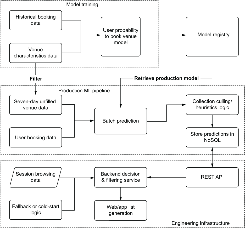
Figure 16.8 Initial serving architecture design

Initially, after building this infrastructure, QA testing looks solid. The response SLA from the NoSQL-backed REST API is performing well, the batch prediction and heuristics logic from the model’s output is optimized for cost, and the fallback logic failover is working flawlessly. The team is ready to start testing the solution with an A/B test.

Unfortunately, the test group’s booking rate is no different from the control group’s rates. Upon analyzing the results, the team finds that fewer than 5% of sessions utilized the predictions, forcing the remaining 95% of page displays to show the fallback logic (which is the same data being shown to the control group). Whoops. To fix this poor performance, the DS team decides to focus on two areas:

• Increasing the number of predictions per user per geographic region
• Increasing the number of regions being predicted per user to cover

This solution dramatically affects their storage costs. What could they have done differently? Figure 16.9 shows a significantly different architecture that could have solved this problem without incurring such a massive cost in processing and storage.

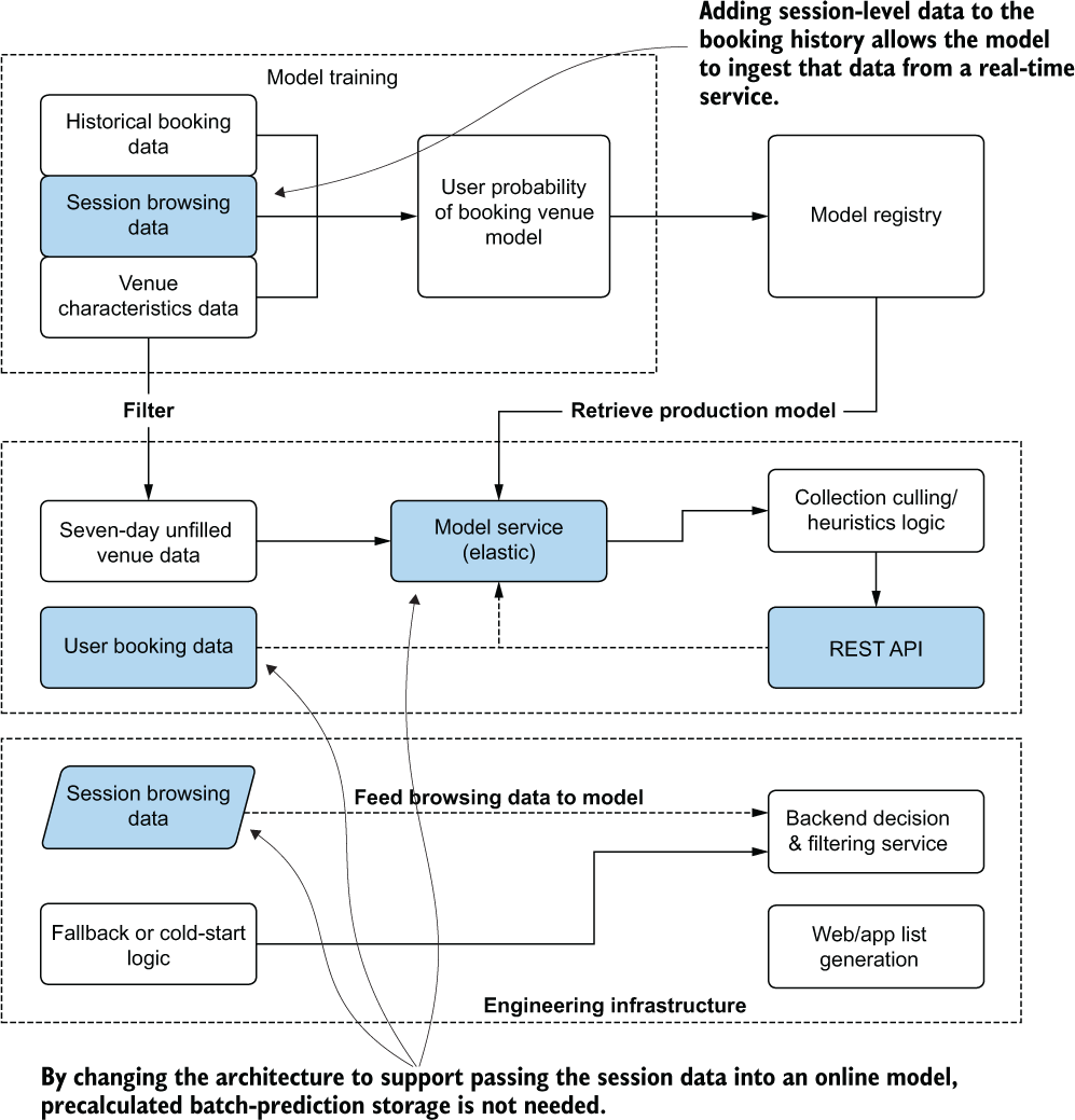
Figure 16.9 A more cost-effective architecture for this use case

While these changes are neither trivial nor, likely, welcome for either the DS team or the site-engineering team, they provide a clear picture about why serving predictions should never be an afterthought for a project. To effectively provide value, several considerations for serving architecture development should be evaluated at the outset of the project. The subsequent subsections cover these considerations and the sorts of architecture required to meet the scenarios.

16.3.1 Determining serving needs

The team in our performance scenario initially failed to design a serving architecture that fully supported the needs of the project. Performing this selection is not a trivial endeavor to get right. However, with a thorough evaluation of a few critical characteristics of a project, the appropriate serving paradigm can be employed to enable an ideal delivery method for predictions.

When evaluating the needs of a project, it’s important to consider the following characteristics of the problem being solved to ensure that the serving design is neither overengineered nor under-engineered.

SLA

The original intention of the team earlier in our scenario was to ensure that their predictions would not interrupt the end user’s app experience. Their design encompassed a precalculated set of recommendations, held in an ultra-low-latency storage system to eliminate the time burden that they assumed would be involved in running a VM-based model service.

SLA considerations are one of the most important facets of an ML architecture design for serving. In general, the solution that is built must consider the budget for serving delays and ensure that for most of the time, this budget is not extended or violated. Regardless of how amazingly a model performs from a prediction accuracy or efficacy standpoint, if it can’t be used or consumed in the amount of time allotted, it’s worthless.

The other consideration that needs to be balanced with that of the SLA requirements is the actual monetary budget. Materialized as a function of infrastructure complexity, the general rule is that the faster a prediction can be served at a larger scale of requests, the more expensive the solution is going to be to host and develop.

Cost

Figure 16.10 shows a relationship between prediction freshness (how long after a prediction is made it is intended to be utilized or acted upon) and the volume of predictions that need to be made as a factor of cost and complexity.

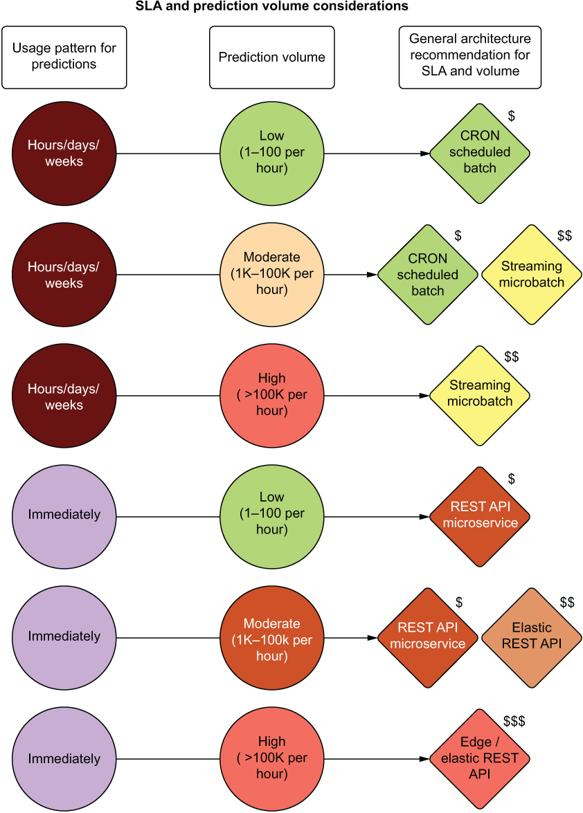
Figure 16.10 Architectural implications to meet SLA and prediction volume needs

The top portion of figure 16.10 shows a traditional paradigm for batch serving. For extremely large production inference volumes, a batch prediction job using Apache Spark Structured Streaming in a trigger-once operation will likely be the cheapest option.

The bottom portion of figure 16.10 involves immediate-use ML solutions. When predictions are intended to be used in a real-time interface, the architecture begins to change dramatically from the batch-inspired use cases. REST API interfaces, elastic scalability of serving containers, and traffic distribution to those services become required as prediction volumes increase.

Recency

Recency, the delay between when feature data is generated and when a prediction can be acted upon, is one of the most important aspects of designing a serving paradigm for a project’s model. SLA considerations are by and large the defining characteristics for choosing a specific serving layer architecture for ML projects. However, edge cases related to recency of the data available for usage in prediction can modify the final scalable and cost-effective design employed for a project.

Depending on a particular situation, the recency of the data and the end use-case for the project can override the general SLA-based design criteria for serving. Figure 16.11 illustrates a set of examples of data recency and consumption layer patterns to show how the architecture can change from the purely SLA-focused designs in figure 16.10.

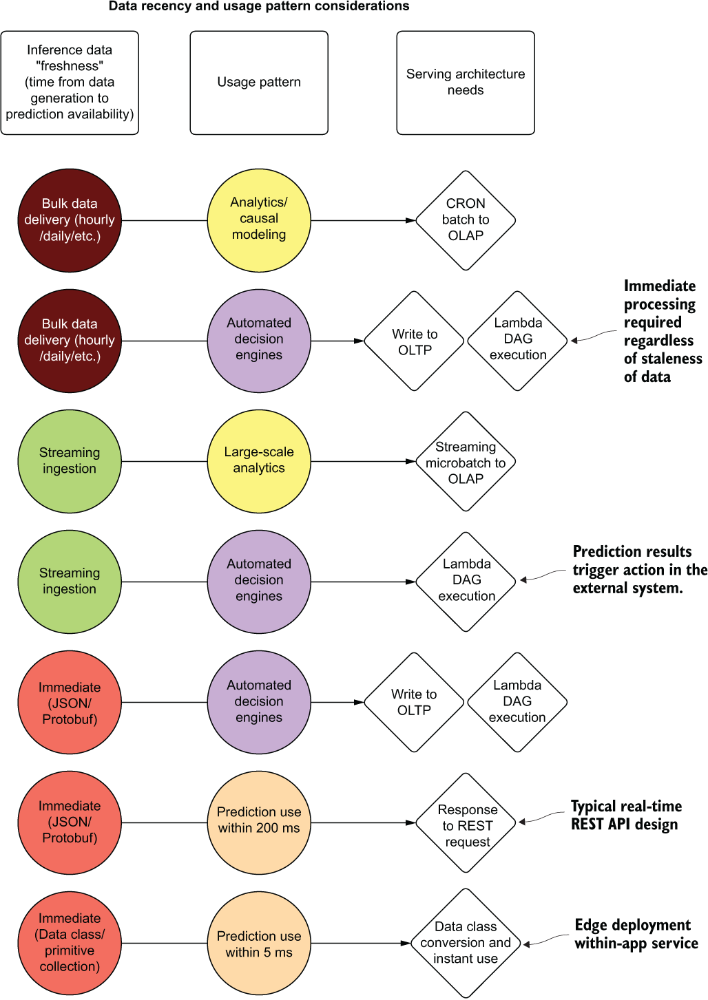
Figure 16.11 The effects of data recency and common usage patterns on serving architectures

These examples are by no means exhaustive. There are as many edge case considerations for serving model predictions as there are nuanced approaches to solving problems with ML. The intention is to open the discussion around which serving solution is appropriate by evaluating the nature of the incoming data, identifying the project’s needs, and seeking the least complex solution possible that addresses the constraints of a project. By considering all aspects of project serving needs (data recency, SLA needs, prediction volumes, and prediction consumption paradigms), the appropriate architecture can be utilized to meet the usage pattern needs while adhering to a design that is only as complex and expensive as it needs to be.

When an ML project’s output is destined for consumption within the walls of a company, the architectural burdens are generally far lower than any other scenario. However, this doesn’t imply that shortcuts can be taken. Utilizing MLOps tools, following robust data management processes, and writing maintainable code are just as critical here as they are for any other serving paradigm. Internal use-case modeling efforts can be classified into two general groups: bulk precomputation and lightweight ad hoc microservice.

Serving from a database or data warehouse

Predictions that are intended for within-workday usage usually utilize a batch prediction paradigm. Models are applied to the new data that has arrived up until the start of the workday, predictions are written to a table (typically in an overwrite mode), and end users within the company can utilize the predictions in an ad hoc manner.

Regardless of the interface method (BI tool, SQL, internal GUI, etc.), the predictions are scheduled to occur at a fixed time (hourly, daily, weekly, etc.), and the only infrastructure burden that the DS team has is ensuring that the predictions are made and make their way to the table. Figure 16.12 shows an example architecture supporting this implementation.

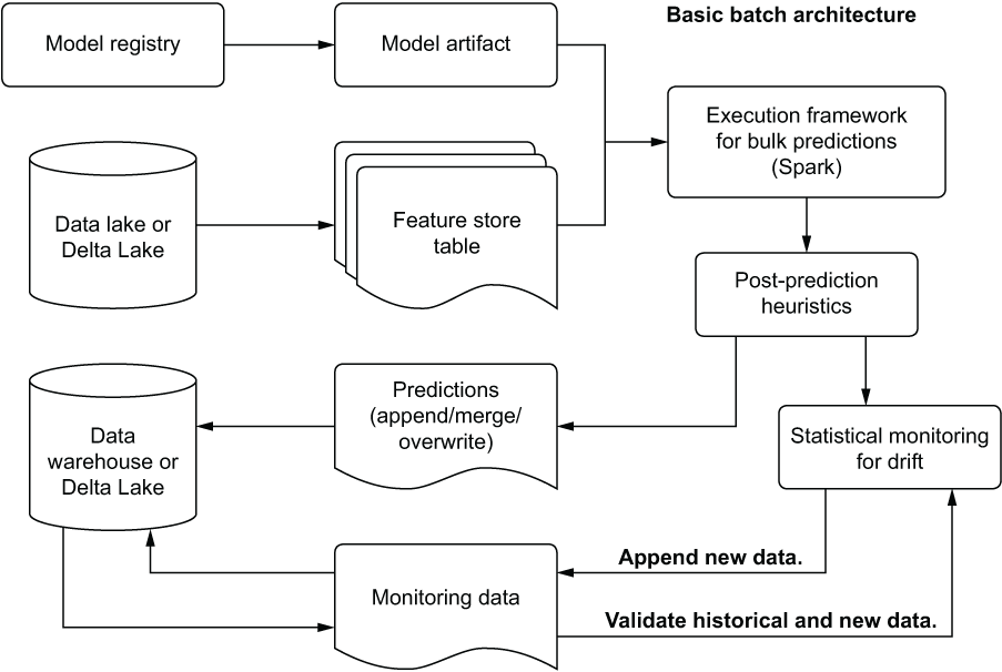
Figure 16.12 Batch serving generic architecture

This architecture is as bare-bones a solution as ML can get. A trained model is retrieved from a registry, data is queried from a source system (preferably from a feature store table), predictions are made, drift monitoring validation occurs, and finally the prediction data is written to an accessible location. For internal use cases on bulk-prediction data, not much more is required from an infrastructure perspective.

Serving from a microservice framework

For internal use cases that rely on more up-to-date predictions on an ad hoc basis or those that allow for a user to specify aspects of the feature vector to receive on-demand predictions (optimization simulations, for instance), precomputation isn’t an option. This paradigm focuses instead on having a lightweight serving layer to host the model, providing a simple REST API interface to ingest data, generate predictions, and return the predictions to the end user.

Most implementations with these requirements are done through BI tools and internal GUIs. Figure 16.13 shows an example of such an architectural setup to support ad hoc predictions.

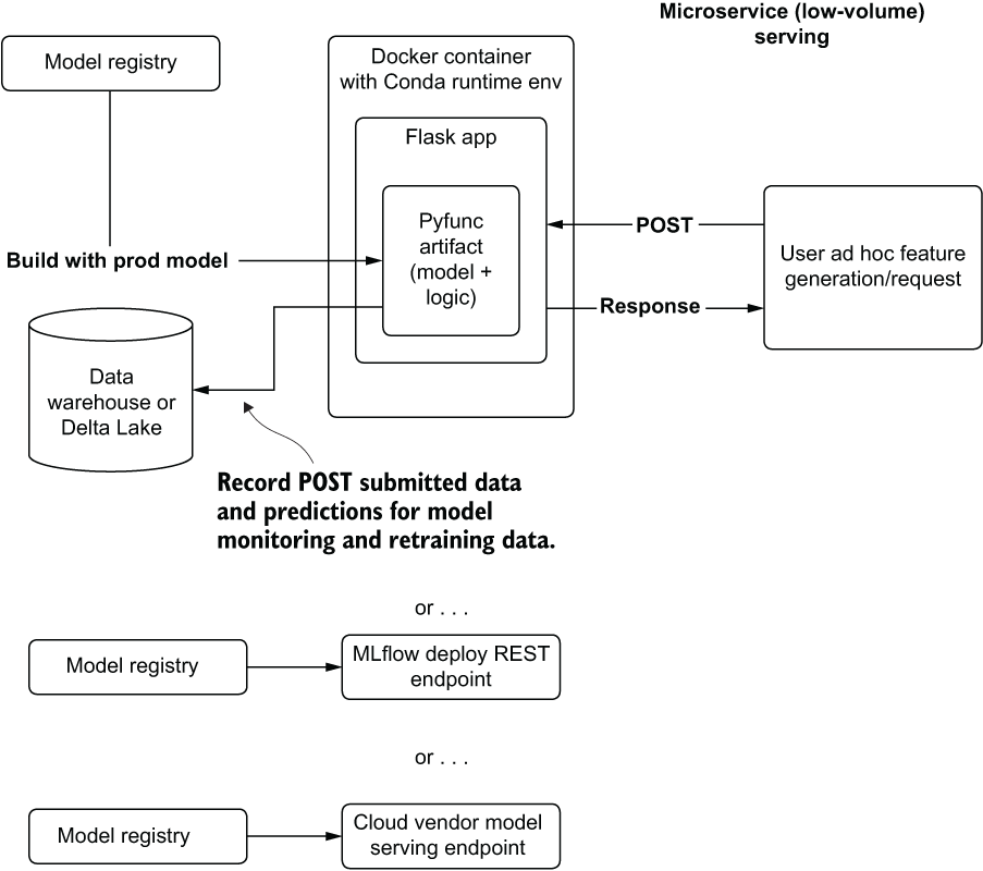
Figure 16.13 Lightweight low-volume REST microservice architecture

The simplicity of this style of deployment is appealing for many use cases of model serving for an internal use-case application. Capable of supporting up to a few dozen requests per second, a lightweight flask deployment of a model can be an attractive alternative to brute-force bulk computing of possible end-use permutations of potential predictions. Although this is technically a real-time serving implementation, it is of critical importance to realize that this is wildly inappropriate for low-latency, high-volume prediction needs or anything that could be customer-facing.

16.3.2 Bulk external delivery

The considerations for bulk external delivery aren’t substantially different from internal use serving to a database or data warehouse. The only material differences between these serving cases are in the realms of delivery time and monitoring of the predictions.

Delivery consistency

Bulk delivery of results to an external party has the same relevancy requirements as any other ML solution. Whether you’re building something for an internal team or generating predictions that will be end-user-customer facing, the goal of creating useful predictions doesn’t change.

The one thing that does change with providing bulk predictions to an outside organization (generally applicable to business-to-business companies) when compared to other serving paradigms is in the timeliness of the delivery. While it may be obvious that a failure to deliver an extract of bulk predictions entirely is a bad thing, an inconsistent delivery can be just as detrimental. There is a simple solution to this, however, illustrated in the bottom portion of figure 16.14.

Figure 16.14 shows the comparison of gated and ungated serving to an external user group. By controlling a final-stage egress from the stored predictions in a scheduled batch prediction job, as well as coupling feature-generation logic to an ETL process governed by a feature store, delivery consistency from a chronological perspective can be guaranteed. While this may not seem an important consideration from the DS perspective of the team generating the predictions, having a predictable data-availability schedule can dramatically increase the perceived professionalism of the serving company.

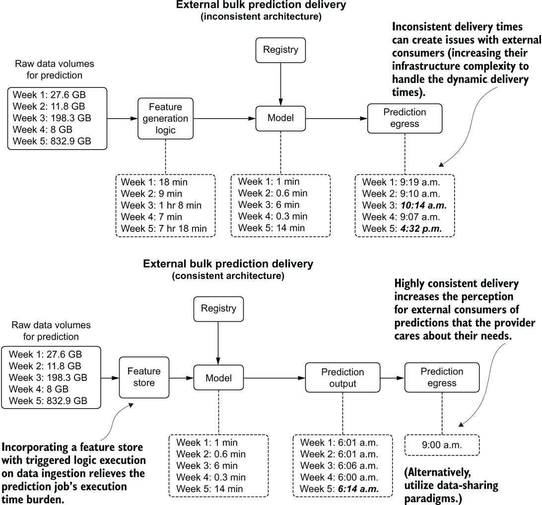
Figure 16.14 Comparison of ungated versus gated batch serving

Quality assurance

An occasionally overlooked aspect of serving bulk predictions externally (external to the DS and analytics groups at a company) is ensuring that a thorough quality check is performed on those predictions.

An internal project may rely on a simple check for overt prediction failures (for example, silent failures are ignored that result in null values, or a linear model predicts infinity). When sending data products externally, additional steps should be done to minimize the chances of end users of predictions finding fault with them. Since we, as humans, are so adept at finding abnormalities in patterns, a few scant issues in a batch-delivered prediction dataset can easily draw the focus of a consumer of the data, deteriorating their faith in the efficacy of the solution to the point of disuse.

In my experience, when delivering bulk predictions external to a team of data specialists, I’ve found it worthwhile to perform a few checks before releasing the data:

• Validate the predictions against the training data:
  • Classification problems—Comparing aggregated class counts
  • Regression problems—Comparing prediction distribution
  • Unsupervised problems—Evaluating group membership counts
• Check for prediction outliers (applicable to regression problems).
• Build (if applicable) heuristics rules based on knowledge from SMEs to ensure that predictions are not outside the realm of possibility for the topic.
• Validate incoming features (particularly encoded ones that may use a generic catchall encoding if the encoding key is previously unseen) to ensure that the data is fully compatible with the model as it was trained.

By running a few extra validation steps on the output of a batch prediction, a great deal of confusion and potential lessening of trust in the final product can be avoided in the eyes of end users.

16.3.3 Microbatch streaming

The applications of streaming prediction paradigms are rather limited. Unable to meet the strict SLA requirements that would force a decision to utilize a REST API service, as well as being complete overkill for small-scale batch prediction needs, streaming prediction holds a unique space in ML serving infrastructure. This niche spot is firmly centered in the needs of a project having a relatively high SLA (measured in the range of whole seconds to weeks) and a large inference dataset size.

The attractiveness of streaming for high SLA needs lies in cost and complexity reduction. Instead of building out a scalable infrastructure to support bulk predictions sent to a REST API service (or similar microservice capable of doing paginated bulk predictions of large data), a simple Apache Spark Structured Streaming job can be configured to allow for draining row-based data from a streaming source (such as Kafka or cloud object storage queue indices) and natively running predictions upon the stream with a serialized model artifact. This helps dramatically reduce complexity, can support streaming-as-batch stateful computation, and can prevent costly infrastructure from having to run when not needed for prediction.

From the perspective of large data sizes, streaming can reduce the required infrastructure size that would otherwise be needed for large dataset predictions in a traditional batch prediction paradigm. By streaming the data through a comparatively smaller cluster of machines than would be required to hold the entire dataset in memory, the infrastructure burden is far less.

This directly translates into lower total cost of ownership for an ML solution with a relatively high SLA. Figure 16.15 shows a simple structured streaming approach to serve predictions at a lower complexity and cost than traditional batch or REST API solutions.

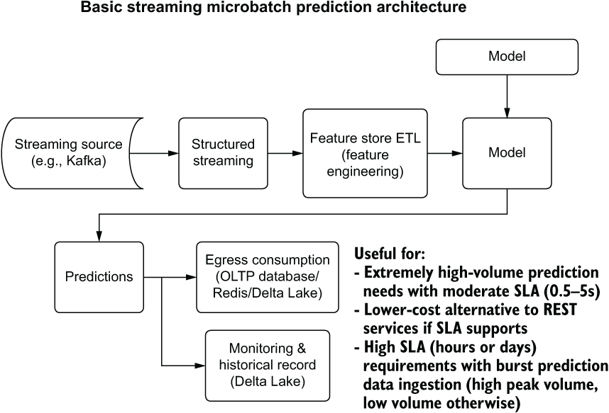
Figure 16.15 A simple structured streaming prediction pipeline architecture

While not able to solve the vast majority of ML serving needs, this architecture still has its place as an attractive alternative to batch prediction for extremely large datasets and to REST APIs when SLAs are not particularly stringent. Implementing this serving methodology is worth it, if it fits this niche, simply for the reduction in cost.

16.3.4 Real-time server-side

The defining characteristic of real-time serving is that of a low SLA. This directly informs the basic architectural design of serving predictions. Any system supporting this paradigm requires a model artifact to be hosted as a service, coupled with an interface for accepting data passed into it, a computational engine to perform the predictions, and a method of returning a prediction to the originating requestor.

The details of implementing a real-time serving architecture can be defined through the classification of levels of traffic, split into three main groupings: low volume, low volume with burst capacity, and high volume. Each requires different infrastructure design and tooling implementation to allow for a high availability and minimally expensive solution.

Low volume

The general architecture for low volume (low-rate requests) is no different from a REST microservice container architecture. Regardless of what REST server is used, what container service is employed to run the application, or what VM management suite is used, the only primary addition for externally facing endpoints is to ensure that the REST service is running on managed hardware. This doesn’t necessarily mean that a fully managed cloud service needs to be used, but the requirement for even a low-volume production service is that the system needs to stay up.

This infrastructure running the container that you’re building should be monitored from not only an ML perspective, but from a performance consideration as well. The memory utilization of the container on the hosting VM, the CPU utilization, network latency, and request failures and retries should all be monitored in real time with a redundant backup available to fail over to if issues arise with fulfilling serving requests.

The scalability and complexity of traffic routing doesn’t become an issue with low-volume solutions (tens to thousands of requests per minute), provided that the SLA requirements for the project are being met, so a simpler deployment and monitoring architecture is called for with low-volume use cases.

Burst volume and high volume

When moving to scales that support burst traffic, integrating elasticity into the serving layer is a critical addition to the architecture. Since an individual VM has only so many threads to process predictions, a flood of requests that come in for prediction and that exceed the execution capacity of a single VM can overwhelm that VM. Unresponsiveness, REST time-outs, and VM instability (potentially crashing) can render a single-VM model deployment unusable. The solution for handling burst volume and high-capacity serving is to incorporate process isolation and routing in the form of elastic load balancing.

Load balancing is, as the name implies, a means of routing requests in a sharded fleet of VMs (duplicated containers of a model serving application). With many containers running in parallel, request loads can be scaled horizontally to support truly staggering volumes of requests. These services (each cloud has its own flavor that essentially does the same thing) are transparent to both the ML team deploying a container and to the end user. With a single endpoint for requests to come into and a single container image to build and deploy, the load-balancing system will ensure that distribution of load burdens happens autonomously to prevent service disruption and instability.

A common design pattern, leveraging cloud-agnostic services, is shown in figure 16.16. Utilizing a simple Python REST framework (Flask) that interfaces with the model artifact from within a container allows for scalable predictions that can support high-volume and burst traffic needs.

This relatively bare-bones architecture is a basic template for an elastically scaling real-time REST-based service to provide predictions. Missing from this diagram are other critical components that we’ve discussed in previous chapters (monitoring of features, retraining triggers, A/B testing, and model versioning), but it has the core components that differentiate a smaller-scale real-time system from that of a service that can handle large traffic volume.

At its core, the load balancer shown in figure 16.16 is what makes the system scale from a single VM’s limit of available cores (putting Gunicorn in front of Flask will allow all cores of the VM to concurrently process requests) to horizontally scaling out to handling hundreds of concurrent predictions (or more). This scalability comes with a caveat, though. Adding this functionality translates to greater complexity and cost for a serving solution.

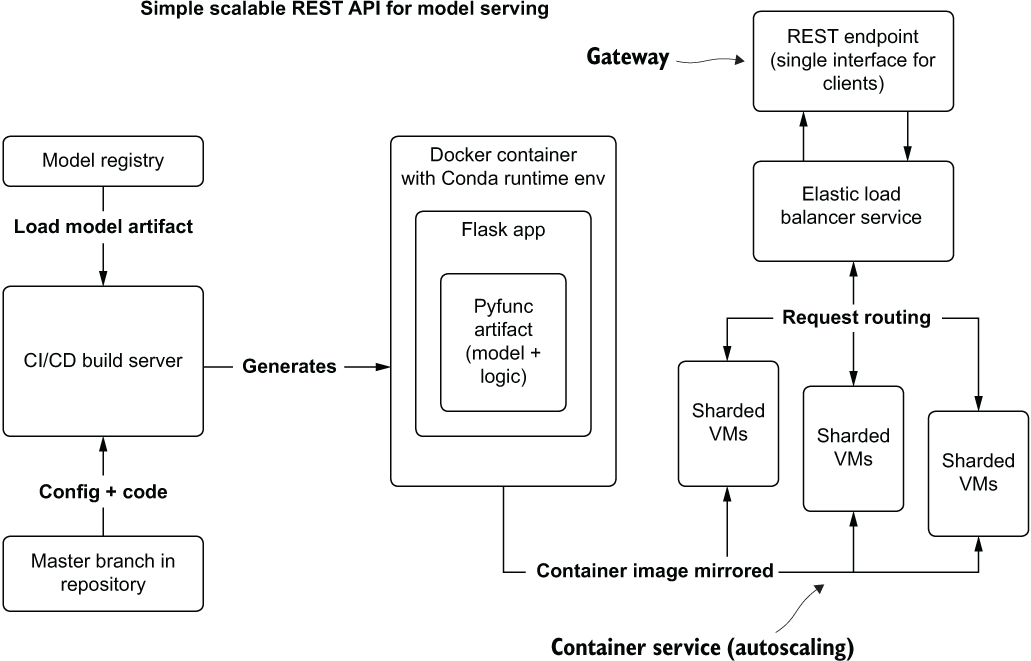
Figure 16.16 Cloud-native REST API model serving architecture

Figure 16.17 shows a more thorough design of a large-scale REST API solution. This architecture can support extremely high rates of prediction traffic and all the services that need to be orchestrated to hit volume, SLA, and analytics use cases for a production deployment.

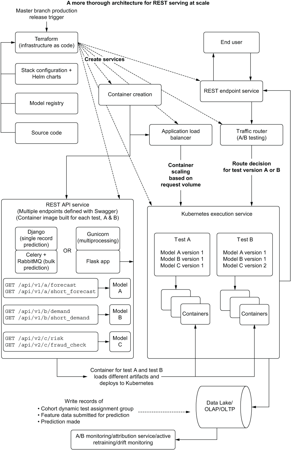
Figure 16.17 Automated infrastructure and services for large-scale REST API model serving

These systems have a lot of components. It’s quite easy for the complexity to grow to the point that dozens of disparate systems are glued together in an application stack to fulfill the needs of the project’s use case. Therefore, it is of the utmost importance to explain not only the complexity involved in supporting these systems, but the cost as well, to the business unit interested in having a solution built that requires this architecture.

Typically, because of this magnitude of complexity, this isn’t a setup that a DS team maintains on its own. DevOps, core engineering, backend developers, and software architects are involved with the design, deployment, and maintenance of services like this. The cloud services bill is one thing to consider for the total cost of ownership, but the other outstanding factor is the human capital investment required to keep a service like this operational constantly.

If your SLA requirements and scale are this complicated, it would be wise to identify these needs as early in the project as possible, be honest about the investment, and make sure that the business understands the magnitude of the undertaking. If they agree that the investment is worth it, go ahead and build it. However, if the prospect of designing and building one of these behemoths is daunting to business leaders, it’s best not to force them into allowing it to be built at the very end of development when so much time and effort has been put into the project.

16.3.5 Integrated models (edge deployment)

Edge deployment is the ultimate stage in low-latency serving for certain use cases. As it deploys a model artifact and all dependent libraries as part of a container image, it has scalability levels that outweigh any other approach. However, this deployment paradigm carries with it a large burden on the part of app developers:

• Deployment of new models or retrained models needs to be scheduled with app deployments and upgrades.
• Monitoring of predictions and generated features is dependent on internet connectivity.
• Heuristics or last-mile corrections to predictions cannot be done server-side.
• Models and infrastructure within the serving container need deeper and more complex integration testing to ensure proper functionality.
• Device capabilities can restrict model complexity, forcing simpler and more lightweight modeling solutions.

For these reasons, edge deployment might not be very appealing for many use cases. The velocity of changes to the models is incredibly low, drift impacts to models can render edge-deployed models irrelevant far more quickly than a new build can be pushed out, and the lack of monitoring available for some end users can provide such intense disadvantages to this paradigm as to leave it inapplicable to most projects. For those that don’t suffer from the detractors for edge deployment, a typical architecture for this serving style is shown in figure 16.18.

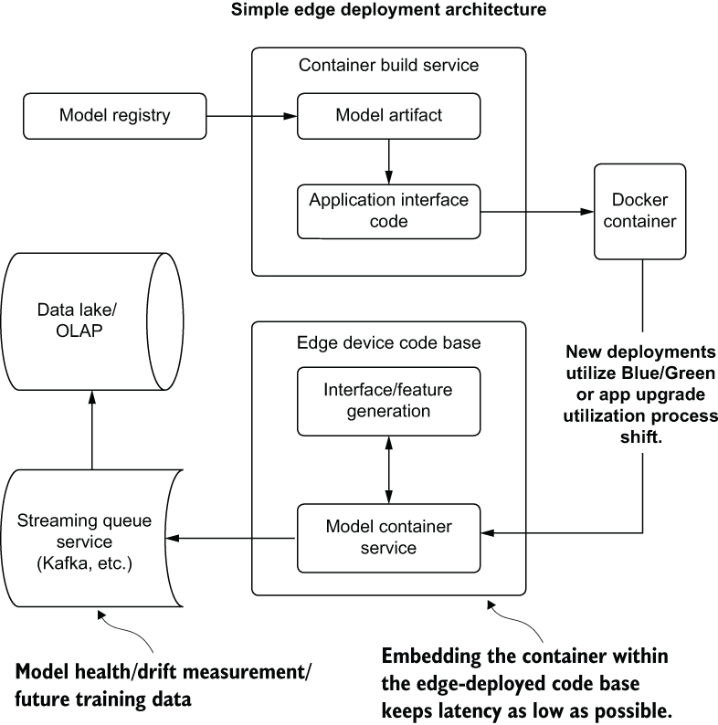
Figure 16.18 A simplified architecture of an edge-deployed model artifact container

As you can see, an edge deployment is tightly coupled to the application code base. Because of the large numbers of required packaged libraries involved in a runtime that can support the predictions being made by the included model, containerizing the artifact prevents the app development team from maintaining an environment that is mirrored to that of the DS team. This can mitigate many of the issues that can plague non-container-based model edge deployments (namely, environment dependency management, language choice standardization, and library synchronization for features in a shared code base).

The projects that can leverage edge deployment, particularly those focused on tasks such as image classification, can dramatically reduce infrastructure costs. The defining aspect of what can qualify for edge deployment is in the state of stationarity in the features being utilized by the model. If the functional nature of the model’s input data will not be changing particularly often (such as with imaging use cases), edge deployment can greatly simplify infrastructure and keep total ownership costs of an ML solution incredibly low.

Summary

• Model registry services will help ensure effective state management of deployed and archived models, enabling effective passive retraining and active retraining solutions without requiring manual intervention.
• Feature stores segregate feature-generation logic from modeling code, allowing for faster retraining processes, reuse of features across projects, and a far simpler method of monitoring for feature drift.
• To choose an appropriate architecture for serving, we must weigh many characteristics of the project: employing the right level of services and infrastructure to support the required SLA, prediction volume, and recency of data to ensure that a prediction service is cost-effective and stable.