9 Modularity for ML: Writing testable and legible code

This chapter covers

• Demonstrating why monolithic script-coding patterns make ML projects more complex
• Understanding the complexity of troubleshooting non-abstracted code
• Applying basic abstraction to ML projects
• Implementing testable designs in ML code bases

Precious few emotions are more soul-crushing than those forced upon you when you’re handed a complex code base that someone else wrote. Reading through a mountain of unintelligible code after being told that you are responsible for fixing, updating, and supporting it is demoralizing. The only worse situation when inheriting a fundamentally broken code base to maintain occurs when your name is the one on the commit history.

This isn’t to say that the code doesn’t work. It may run perfectly fine. The fact that code runs isn’t the issue. It’s that a human can’t easily figure out how(or, more disastrously, why) it works. I believe this problem was most eloquently described by Martin Fowler in 2008:

Any fool can write code that a computer can understand. Good programmers write code that humans can understand.

A large portion of ML code is not aligned with good software engineering practices. With our focus on algorithms, vectors, indexers, models, loss functions, optimization solvers, hyperparameters, and performance metrics, we, as a profession of practitioners, generally don’t spend much time adhering to strict coding standards. At least, most of us don’t.

I can proudly claim that I was one such person for many years, writing some truly broken code (it worked when I released it, most of the time). Focused solely on eking the slightest of accuracy improvements or getting clever with feature-engineering tasks, I would end up creating a veritable Frankenstein’s monster of unmaintainable code. To be fair to that misunderstood reanimated creature, some of my early projects were far more horrifying. (I wouldn’t have blamed my peers if they chased me with torches and pitchforks.)

This chapter and the next are devoted to the lessons in coding standards that I’ve learned over the years. It is by no means an exhaustive treatise on the topic of software engineering; there are books for that. Rather, these are the most important aspects that I’ve learned in order to create simpler and easier-to-maintain code bases for ML project work. We will cover these best practices in five key areas, as shown in figure 9.1.

The sections in this chapter, reflected in figure 9.1, demonstrate examples of the horrible things that I’ve done, the terrifying elements that I’ve seen in others’ code, and, most important, ways to address them. Our goal in this chapter is to avoid the Frankenstein’s monster of convoluted and overly complex code.

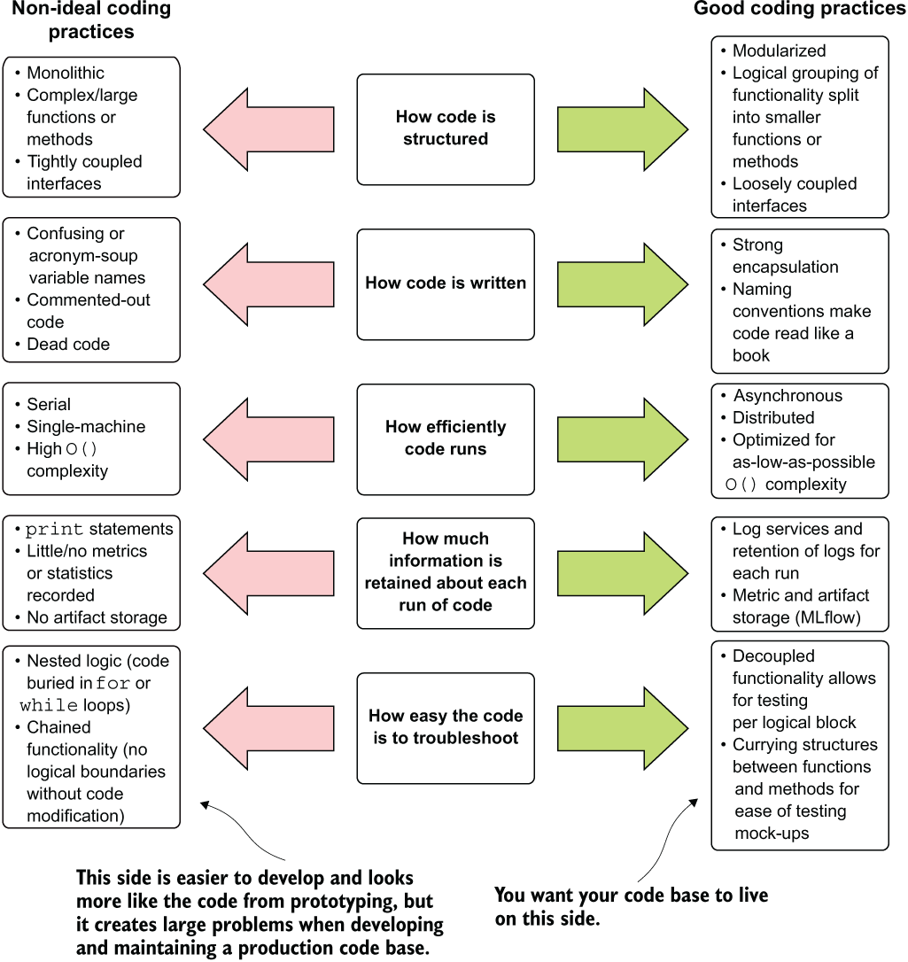
Figure 9.1 Comparing extremes of coding practices for ML project work

To make things easier, we’re going to look at a single relatively simple example throughout this chapter, something that we should all be rather familiar with: a distribution estimation for univariate data. We’ll stick with this example because it is simple and approachable. We’ll look at the same effective solution through the lens of different programming problems, discussing how important it is to focus on maintainability and utility above all other considerations.

9.1 Understanding monolithic scripts and why they are bad

Inheritance, in the world of computing, can mean a few different things. The topic first comes to mind when thinking of crafting extensible code through abstraction (code reuse in object-oriented design to reduce copied functionality and decrease complexity). While this type of inheritance is undeniably good, a different type of inheritance can range from good to nightmarish. This is the inheritance we get when assuming responsibility for someone else’s code base.

Let’s imagine that you start at a new company. After indoctrination is done, you’re given a token to access the DS repository (repo). This moment of traversing the repo for the first time is either exciting or terrifying, depending on the number of times you’ve done this before. What are you going to find? What have your predecessors at this company built? How easy is the code going to be to debug, modify, and support? Is it filled with technical debt? Is it consistent in style? Does it adhere to language standards?

At first glance, you feel a sinking in your stomach as you look through the directory structure. There are dozens of directories, each with a project name. Within each of these directories is a single file. You know you are in for a world of frustration in figuring out how any of these monolithic and messy scripts work. Any on-call support you’ll be tasked with providing for these is going to be incredibly challenging. Each issue that comes up, after all, will involve reverse engineering these confusing and complicated scripts for even the most trivial of errors that occur.

9.1.1 How monoliths come into being

If we were to dig into the commit history of our new team’s repository, we’d likely find a seamless transition from prototype to experimentation. The first commit would likely be the result of a bare-bones experiment, filled with TODO comments and placeholder functionality. As we move through the commit history, the script begins to take shape, piece by piece, finally arriving at the production version of the code that you see in the master branch.

The problem here is not that scripting was used. The vast majority of professional ML engineers, myself included, do our prototyping and experimentation in notebooks (scripts). The dynamic nature of notebooks and the ability to rapidly try out new ideas makes them an ideal platform for this stage of work. Upon accepting a prototype as a path to develop, however, all of that prototype code is thrown out in favor of creating modularized code during MVP development.

The evolution of a script from a prototype is understandable. ML development is notorious for having countless changes, needing rapid feedback of results, and pivoting dramatically in approaches during the MVP phase. Even during early phases, however, the code can be structured such that it is much easier to decouple functionality, abstract away complexity, and create a more testable (and debug-friendly) code base.

The way a monolithic production code base comes into being is by shipping a prototype to production. This is never advisable.

9.1.2 Walls of text

If there was one thing that I learned relatively early in my career as a data scientist, it was that I truly hate debugging. It wasn’t the act of tracking down a bug in my code that frustrated me; rather, it was the process that I had to go through to figure out what went wrong in what I was telling the computer to do.

Like many DS practitioners at the start of their career, when I began working on solving problems with software, I would write a lot of declarative code. I wrote my solutions much in the way that I logically thought about the problem (“I pull my data, then I do some statistical tests, then I make a decision, then I manipulate the data, then I put it in a vector, then into a model . . . ”). This materialized as a long list of actions that flowed directly, one into another. What this programming model meant in the final product was a massive wall of code with no separation or isolation of actions, let alone encapsulation.

Finding the needle in the haystack for any errors in code written in that manner is an exercise in pure, unadulterated torture. The architecture of the code was not conducive to allowing me to figure out which of the hundreds of steps contained therein was causing an issue.

Troubleshooting walls of text (WoT, pronounced What?!) is an exercise in patience that bears few parallels in depth and requisite effort. If you’re the original author of such a display of code, it’s an annoying endeavor (you have no one to hate other than yourself for creating the monstrosity), depressing activity (see prior comment), and time-consuming slog that can be so easily avoided—provided you know how, what, and where to isolate elements within your ML code.

If written by someone else, and you’re the unfortunate heir to the code base, I extend to you my condolences and a hearty “Welcome to the club.” Perhaps a worthy expenditure of your time after fixing the code base would be to mentor the author, provide them with an ample reading list, and help them to never produce such rage-inducing code again.

To have a frame of reference for our discussion, let’s take a look at what one of these WoTs could look like. While the examples in this section are rather simplistic, the intention is to imagine what a complete end-to-end ML project would look like in this format, without having to read through hundreds of lines. (I imagine that you wouldn’t like to flip through dozens of pages of code in a printed book.)

Listing 9.1 presents a relatively simple block of script that is intended to be used to determine the nearest standard distribution type to a passed-in series of continuous data. The code contains some normalcy checks at the top, comparisons to the standard distributions, followed by the generation of a plot.

NOTE The code examples in this chapter are provided in the accompanying repository for this book. However, I do not recommend that you run them. They take a very long time to execute.

Listing 9.1 A wall-of-text script

import warnings as warn
import pandas as pd
import numpy as np
import scipy.stats as stat
from scipy.stats import shapiro, normaltest, anderson
import matplotlib.pyplot as plt
from statsmodels.graphics.gofplots import qqplot
 
data = pd.read_csv('/sf-airbnb-clean.csv')
series = data['price']
shapiro, pval = shapiro(series)                                          ❶
print('Shapiro score: ' + str(shapiro) + ' with pvalue: ' + str(pval))   ❷
dagastino, pval = normaltest(series)                                     ❸
print("D'Agostino score: " + str(dagastino) + " with pvalue: " + str(pval))
anderson_stat, crit, sig = anderson(series)
print("Anderson statistic: " + str(anderson_stat))
anderson_rep = list(zip(list(crit), list(sig)))
for i in anderson_rep:
    print('Significance: ' + str(i[0]) + ' Crit level: ' + str(i[1]))
bins = int(np.ceil(series.index.values.max()))                           ❹
y, x = np.histogram(series, 200, density=True)
x = (x + np.roll(x, -1))[:-1] / 2.                                       ❺
bl = np.inf                                                              ❻
bf = stat.norm
bp = (0., 1.)
with warn.catch_warnings():
    warn.filterwarnings('ignore')
    fam = stat._continuous_distns._distn_names
    for d in fam:
        h = getattr(stat, d)                                             ❼
        f = h.fit(series)
        pdf = h.pdf(x, loc=f[-2], scale=f[-1], *f[:-2])
        loss = np.sum(np.power(y - pdf, 2.))
        if bl > loss > 0:
            bl = loss
            bf = h
            bp = f
start = bf.ppf(0.001, *bp[:-2], loc=bp[-2], scale=bp[-1])
end = bf.ppf(0.999, *bp[:-2], loc=bp[-2], scale=bp[-1])
xd = np.linspace(start, end, bins)
yd = bf.pdf(xd, loc=bp[-2], scale=bp[-1], *bp[:-2])
hdist = pd.Series(yd, xd)
with warn.catch_warnings():
    warn.filterwarnings('ignore')
    with plt.style.context(style='seaborn'):
        fig = plt.figure(figsize=(16,12))
        ax = series.plot(kind='hist', bins=100, normed=True, alpha=0.5, label='Airbnb SF Price', legend=True)                               ❽
        ymax = ax.get_ylim()
        xmax = ax.get_xlim()
        hdist.plot(lw=3, label='best dist ' + bf.__class__.__name__, legend=True, ax=ax)
        ax.legend(loc='best')
        ax.set_xlim(xmax)
        ax.set_ylim(ymax)
qqplot(series, line='s')

❶ pval? That’s not a standard naming convention. It should be p_value_shapiro or something similar.

❷ String concatenation is difficult to read, can create issues in execution, and requires more things to type. Don’t do it.

❸ Mutating the variable pval makes the original one from shapiro inaccessible for future usage. This is a bad habit to adopt and makes more complex code bases nigh impossible to follow.

❹ With such a general variable name, we have to search through the code to find out what this is for.

❺ Mutating x here makes sense, but again, we have no indication of what this is for.

❻ bl? What is that?! Abbreviations don’t help the reader understand what is going on.

❼ All of these single-letter variable names are impossible to figure out without reverse engineering the code. It may make for concise code, but it’s really hard to follow. With a lack of comments, this shorthand becomes difficult to read.

❽ All of these hardcoded variables (the bins in particular) mean that if this needs to be adjusted, the source code needs to be edited. All of this should be abstracted in a function.

My most sincere apologies for what you just had to look at. Not only is this code confusing, dense, and amateurish, but it’s written in such a way that its style is approaching intentional obfuscation of functionality.

The variable names are horrific. Single-letter values? Extreme shorthand notation in variable names? Why? It doesn’t make the program run faster. It just makes it harder to understand. Tunable values are hardcoded, requiring modification of the script for each test, which can be exceedingly prone to errors and typos. No stopping points are set in the execution that would make it easy to figure out why something isn’t working as intended.

9.1.3 Considerations for monolithic scripts

Aside from being hard to read, listing 9.1’s biggest flaw is that it’s monolithic. Although it is a script, the principles of WoT development can apply to both functions and methods within classes. This example comes from a notebook, which increasingly is the declarative vehicle used to execute ML code, but the concept applies in a general sense.

Having too much logic within the bounds of an execution encapsulation creates problems (since this is a script run in a notebook, the entire code is one encapsulated block). I invite you to think about these issues through the following questions:

• What would it look like if you had to insert new functionality in this block of code?
• Would it be easy to test if your changes are correct?
• What if the code threw an exception?
• How would you go about figuring out what went wrong with the code from an exception being thrown?
• What if the structure of the data changed? How would you go about updating the code to reflect those changes?

Before we get into answering some of these questions, let’s look at what this code actually does. Because of the confusing variable names, dense coding structure, and tight coupling of references, we would have to run it to figure out what it’s doing. The next listing shows the first aspect of listing 9.1.

Listing 9.2 Stdout results from listing 9.1 print statements

Shapiro score: 0.33195996284484863 with pvalue: 0.0     ❶
D'Agostino score: 14345.798651770001 with pvalue: 0.0   ❷
Anderson statistic: 1022.1779688188954
Significance: 0.576 Crit level: 15.0                    ❸
Significance: 0.656 Crit level: 10.0
Significance: 0.787 Crit level: 5.0
Significance: 0.917 Crit level: 2.5
Significance: 1.091 Crit level: 1.0

❶ That is, perhaps, a few too many significant digits to be useful.

❷ These pvalue elements are potentially confusing. Without some sort of explanation of what they signify, a user has to look up these tests in the API documentation to understand what they are.

❸ With no explanation about these significances and critical levels, this data is meaningless to anyone unfamiliar with the Anderson-Darling test.

This code is doing normalcy tests for a univariate series (a column within a DataFrame here). These are definitely worthwhile tests to conduct on a target variable for a regression problem. The image shown in figure 9.2 is the result of the first of the plots that are generated by the remainder of the script (apart from the very last line).

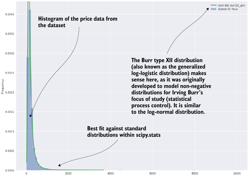
Figure 9.2 The first plot that is generated from listing 9.1

NOTE Chapter 8 covered the power of logging information to MLflow and other such utilities, and how bad of an idea it is to print important information to stdout. However, this example is the exception. MLflow stands as a comprehensive utility tool that aids in model-based experimentation, development, and production monitoring. For our example, in which we are performing a one-off validation check, utilizing a tool like MLflow is simply not appropriate. If the information that we need to see is relevant for only a short period of time (while deciding a particular development approach, for instance), maintaining an indefinite persistence of this information is confusing and pointless.

Figure 9.3 shows the last plot that is generated from listing 9.1.

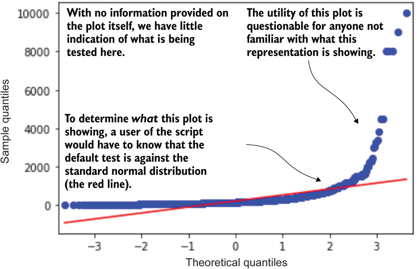
Figure 9.3 The tacked-on-at-the-end plot generation from listing 9.1

This quantile-quantile plot is a similarly useful exploratory aid in determining the normalcy (or goodness of fit to different distributions) by plotting the quantile values from a series against those of another series. In this example, the quantiles of the price series from the dataset are plotted against those of the standard normal distribution.

With no callout in the code or indication of what this plot is, however, the end user of this script can be left a bit confused about what is going on. It’s rarely ever a good practice to place evaluations into code in this manner; they are easily overlooked, and users may be perplexed about why they are included in that location in the code.

Let’s pretend for a moment that we aren’t restricted to the medium of print here. Let’s say that instead of a simple statistical analysis of a single target variable example, we are looking at a full project written as a monolithic script, as was shown in listing 9.1. Something on the order of, say, 1,500 lines. What would happen if the code broke? Can we clearly see and understand everything that’s happening in the code in such a format? Where would we begin to troubleshoot the issue?

9.2 Debugging walls of text

If we fast-forward a bit in our theoretical new job, after having seen the state of the code base, we’d eventually be in the position of maintaining it. Perhaps we were tasked with integrating a new feature into one of the preexisting scripts. After reverse engineering the code, and commenting it for our own understanding, we progress to putting in the new functionality. The only way, at this point, to test our code is to run the entire script.

We’re inevitably going to have to work through some bugs in the process of changing the script to accommodate the new features. If we’re dealing with a script or notebook environment with a long list of actions being taken in succession, how can we troubleshoot what went wrong with the code? Figure 9.4 shows the troubleshooting process that would have to happen to correct an issue in the WoT in listing 9.1.

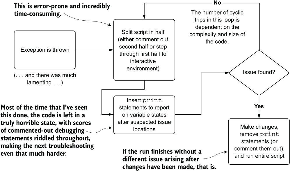
Figure 9.4 The time-consuming and patience-testing process of binary troubleshooting complicates (not necessarily complex) monolithic code bases.

This process, as frustrating as it is to go through, is complicated enough without having poor variable names and confusing shorthand notation as in listing 9.1. The more difficult the code is to read and follow, the deeper the cognitive load required, both to select binary boundary points for isolation while testing the code and to figure out which variable states will need to be reported out to stdout.

This halving process of evaluating and testing portions of the code means that we’re having to actually change the source code to do our testing. Whether we’re adding print statements, debugging comments, or commenting out code, a lot of work is involved in testing faults with this paradigm. Mistakes will likely be made, and there is no guarantee that you won’t add in a new issue through manipulating the code in this way.

Surely, there must be a better way to organize code (complex or not) to reduce the levels of complication. Listing 9.3 shows an alternative in the form of an OO version of the script from listing 9.1.

9.3 Designing modular ML code

After going through such a painful exercise of finding, fixing, and validating our change to this massive script, we’ve hit our breaking point. We communicate to the team that the code’s technical debt is too high, and we need to pay it down before any other work continues. Accepting this, the team agrees to breaking up the script by functionality, abstracting the complexity into smaller pieces that can be understood and tested in isolation.

Before we look at the code, let’s analyze the script to see its main groupings of functionality. This functionality-based analysis can help inform what methods to create in order to achieve functionality isolation (aiding our ability to troubleshoot, test, and insert new features in the future). Figure 9.5 illustrates the core functionality contained within the script and how we can extract, encapsulate, and create single-purpose code groupings to define what belongs in our methods.

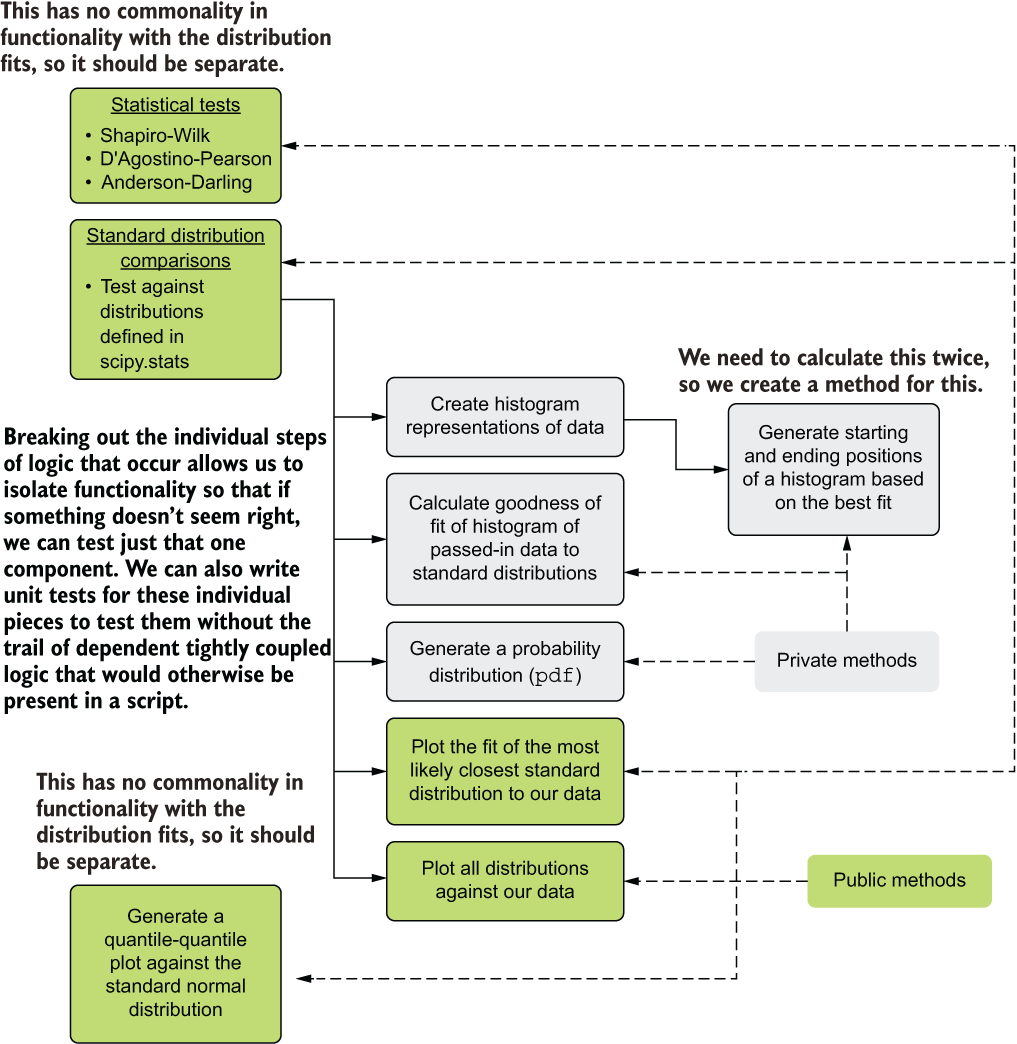
Figure 9.5 Code architecture refactoring for listing 9.1

This structural and functional analysis of the code helps us rationalize the elements of common functionality. From this inspection, elements are identified, isolated, and encapsulated to aid in both legibility (to help us, the humans) and maintainability (troubleshooting and extensibility) of the code. Notice the private (internal functionality that the end user doesn’t need to use to get value from the module) and public (the user-facing methods that will generate specific actions from the code based on what they need) methods. Hiding internal functionality from users of this module will help reduce the cognitive load placed on the user, while minimizing the code complexity as much as possible.

Now that we have a plan for refactoring the code from the nigh-unintelligible script into something easier to follow and maintain, let’s look at the final product of the refactoring and modularization in the next listing.

Listing 9.3 An object-oriented version of the scripted code from listing 9.1

 
import warnings as warn
import pandas as pd
import numpy as np
import scipy
import scipy.stats as stat
from scipy.stats import shapiro, normaltest, anderson
import matplotlib.pyplot as plt
from statsmodels.graphics.gofplots import qqplot
 
class DistributionAnalysis(object):                                          ❶
 
    def __init__(self, series, histogram_bins, **kwargs):                    ❷
        self.series = series
        self.histogram_bins = histogram_bins
        self.series_name = kwargs.get('series_name', 'data')
        self.plot_bins = kwargs.get('plot_bins', 200)
        self.best_plot_size = kwargs.get('best_plot_size', (20, 16))
        self.all_plot_size = kwargs.get('all_plot_size', (24, 30))
        self.MIN_BOUNDARY = 0.001                                            ❸
        self.MAX_BOUNDARY = 0.999
        self.ALPHA = kwargs.get('alpha', 0.05)
 
    def _get_series_bins(self):                                              ❹
        return int(np.ceil(self.series.index.values.max()))
 
    @staticmethod                                                            ❺
    def _get_distributions():
        scipy_ver = scipy.__version__                                        ❻
        if (int(scipy_ver[2]) >= 5) and (int(scipy_ver[4:]) > 3):
            names, gen_names = stat.get_distribution_names(stat.pairs, stat.rv_continuous)
        else:
            names = stat._continuous_distns._distn_names
        return names
 
    @staticmethod                                                            ❼
    def _extract_params(params):
        return {'arguments': params[:-2], 'location': params[-2], 'scale': 
          params[-1]}                                                        ❽
    @staticmethod
    def _generate_boundaries(distribution, parameters, x):                   ❾
        args = parameters['arguments']
        loc = parameters['location']
        scale = parameters['scale']
        return distribution.ppf(x, *args, loc=loc, scale=scale) if args else distribution.ppf(x, loc=loc, scale=scale)                               ❿
 
    @staticmethod
    def _build_pdf(x, distribution, parameters):                             ⓫
        if parameters['arguments']:
            pdf = distribution.pdf(x, loc=parameters['location'], 
              scale=parameters['scale'], *parameters['arguments'])
        else:
            pdf = distribution.pdf(x, loc=parameters['location'], 
              scale=parameters['scale'])
        return pdf
 
    def plot_normalcy(self):
        qqplot(self.series, line='s')                                        ⓬
 
    def check_normalcy(self):                                                ⓭
        def significance_test(value, threshold):                             ⓮
            return "Data set {} normally distributed from".format('is' if value 
              > threshold else 'is not')
        shapiro_stat, shapiro_p_value = shapiro(self.series)
        dagostino_stat, dagostino_p_value = normaltest(self.series)
        anderson_stat, anderson_crit_vals, anderson_significance_levels = 
          anderson(self.series)
        anderson_report = list(zip(list(anderson_crit_vals), 
          list(anderson_significance_levels)))
        shapiro_statement = """Shapiro-Wilk stat: {:.4f}
        Shapiro-Wilk test p-Value: {:.4f}
        {} Shapiro-Wilk Test""".format(
            shapiro_stat, shapiro_p_value, significance_test(shapiro_p_value, 
              self.ALPHA))
        dagostino_statement = """
D'Agostino stat: {:.4f}
        D'Agostino test p-Value: {:.4f}
        {}  D'Agostino Test""".format(
            dagostino_stat, dagostino_p_value, significance_test(dagostino_p_value, self.ALPHA))
        anderson_statement = '
Anderson statistic: {:.4f}'.format(anderson_stat)
        for i in anderson_report:
            anderson_statement = anderson_statement + """
            For signifance level {} of Anderson-Darling test: {} the evaluation. 
              Critical value: {}""".format(
                i[1], significance_test(i[0], anderson_stat), i[0])
        return "{}{}{}".format(shapiro_statement, dagostino_statement, 
          anderson_statement)
 
    def _calculate_fit_loss(self, x, y, dist):                                   ⓯
        with warn.catch_warnings():
            warn.filterwarnings('ignore')
            estimated_distribution = dist.fit(x)
            params = self._extract_params(estimated_distribution)
            pdf = self._build_pdf(x, dist, params)
        return np.sum(np.power(y - pdf, 2.0)), estimated_distribution
 
    def _generate_probability_distribution(self, distribution, parameters, bins):⓰
        starting_point = self._generate_boundaries(distribution, parameters, 
          self.MIN_BOUNDARY)
        ending_point = self._generate_boundaries(distribution, parameters, 
          self.MAX_BOUNDARY)
        x = np.linspace(starting_point, ending_point, bins)
        y = self._build_pdf(x, distribution, parameters)
        return pd.Series(y, x)
 
    def find_distribution_fit(self):                                           ⓱
        y_hist, x_hist_raw = np.histogram(self.series, self.histogram_bins, 
          density=True)
        x_hist = (x_hist_raw + np.roll(x_hist_raw, -1))[:-1] / 2.
        full_distribution_results = {}                                         ⓲
        best_loss = np.inf
        best_fit = stat.norm
        best_params = (0., 1.)
        for dist in self._get_distributions():
            histogram = getattr(stat, dist)
            results, parameters = self._calculate_fit_loss(x_hist, y_hist, 
              histogram)
            full_distribution_results[dist] = {'hist': histogram,
                                               'loss': results,
                                               'params': {
                                                   'arguments': parameters[:-2],
                                                   'location': parameters[-2],
                                                   'scale': parameters[-1]
                                               }}
            if best_loss > results > 0:
                best_loss = results
                best_fit = histogram
                best_params = parameters
        return {'best_distribution': best_fit,
                'best_loss': best_loss,
                'best_params': {
                    'arguments': best_params[:-2],
                    'location': best_params[-2],
                    'scale': best_params[-1]
                },
                'all_results': full_distribution_results
                }
 
    def plot_best_fit(self):                                                 ⓲
        fits = self.find_distribution_fit()
        best_fit_distribution = fits['best_distribution']
        best_fit_parameters = fits['best_params']
        distribution_series = self._generate_probability_distribution(best_fit_distribution,        best_fit_parameters,                                                         self._get_series_bins())
        with plt.style.context(style='seaborn'):
            fig = plt.figure(figsize=self.best_plot_size)
            ax = self.series.plot(kind='hist', bins=self.plot_bins, normed=True,
                                  alpha=0.5, label=self.series_name, 
                                  legend=True)
            distribution_series.plot(lw=3,
➥label=best_fit_distribution.__class__.__name__, legend=True, ax=ax)
            ax.legend(loc='best')
        return fig
 
    def plot_all_fits(self):                                                 ⓴
 
        fits = self.find_distribution_fit()
        series_bins = self._get_series_bins()
 
        with warn.catch_warnings():
            warn.filterwarnings('ignore')
            with plt.style.context(style='seaborn'):
                fig = plt.figure(figsize=self.all_plot_size)
                ax = self.series.plot(kind='hist', 
                                      bins=self.plot_bins, 
                                      normed=True, 
                                      alpha=0.5,
                                      label=self.series_name, 
                                      legend=True)
                y_max = ax.get_ylim()
                x_max = ax.get_xlim()
                for dist in fits['all_results']:
                    hist = fits['all_results'][dist]
                    distribution_data = self._generate_probability_distribution(
                      hist['hist'], hist['params'], series_bins)
                    distribution_data.plot(lw=2, label=dist, alpha=0.6, ax=ax)
                ax.legend(loc='best')
                ax.set_ylim(y_max)
                ax.set_xlim(x_max)
        return fig

❶ Encapsulates the entire module as a class since all of the functionality within is focused on distribution analysis

❷ Passes in a **kwargs argument so defined defaults within the class initialization method can be overridden with a key-value combination (the script had these all hardcoded)

❸ These values are left as static but could be wrapped into kwargs overrides if needed.

❹ Private utility method to keep the callee locations cleaner and easier to read

❺ A static method is effectively an encapsulated function; no references to the initialized arguments are passed into the class, nor are there dependencies on any other methods. Most code bases have quite a few of these, and it’s considered a better practice than defining global functions to prevent issues with mutable state in a global context.

❻ Version checks switch statement since the SciPy API changed (a frequent occurrence in Python open source libraries as these libraries are improved over time). Newer versions of SciPy have protected the access to the distribution listing and have created an access method to retrieve them

❼ Method for extracting the parameters from a distribution fit, putting them into a dictionary structure (this is known as currying, an eponymous reference to Haskell Curry, which condenses complex return types into a single reference to make code much cleaner).

❽ Recall that this exact reference logic was copied multiple times throughout listing 9.1. Providing a single reference to extract this information reduces the chances of typo-induced bugs in code, which are frustrating to troubleshoot.

❾ Private method to generate the starting and ending points of the generated standard histograms through the percent point function (the inverse of the cumulative distribution function) for a distribution

❿ Switch logic to handle some distributions requiring only two arguments (location and scale), while others require additional arguments

⓫ Private method for building the probability density function (pdf) based on the fit parameters found. The switch conditional is due to the varying number of arguments among the distribution families.

⓬ A public method for generating the Q-Q plot comparing the series against the standard normal distribution. For future work, this could be expanded or refactored to allow plotting against any distribution within scipy.stats.

⓭ The stdout print functions for reporting on normalcy tests to the three primary families. The interpolation here is a bit different than in the script, and the human-readable nature of the decision of normalcy based on a passed-in alpha significance level makes the final report more interpretable and less prone to error in making assumptions about the series.

⓮ A method-private method. Since this functionality is solely intended to make the code easier to read and less dense, and has no external uses, making it private within this method is a preferred methodology.

⓯ Private method to score the fit of the histogram of the data series under test to the standard histograms in scipy.stats, using SSE

⓰ Private method for generating the pdf and converting it to a series of data points to compare against the raw passed-in data series

⓱ Primary raw method for finding the closest (and all other) standard distributions to the series passed in. From an end-user perspective, exposing the raw data from the results of a module is sometimes worthwhile (often marked as a developer API) so that the user can use such data to perform additional actions.

⓲ Currying again so we don’t have to return a complex n-valued tuple as a return statement. Dictionaries in Python (and case classes in Scala) are preferable to positional-encoded return statements to make debugging and end-user experiences much more seamless, even if it means more typing for the developer of the module.

⓲ Public method for plotting the best fit found to the series data passed in for evaluation to the class

⓴ Additional method to plot all the distributions against the passed-in series data as an aid to visualize similarities between standard distributions

This code is functionally identical to that of the script. It produces the same results in the same amount of runtime and will just-in-time (JIT) compile to the exact same byte code as the script in listing 9.1 (minus the additional method for plotting all standard reference distributions against the series data). The primary difference in this code is in its utility.

While there are significantly more lines of code here than in the script, we now have isolation in the processing of the core logic of the code. We can walk through the code, method by method, to trace any issues that might arise, aiding any troubleshooting that may need to be done by a very large degree. We also now have the ability to unit test the code. With data mock-ups of predictable and readily understandable data, we can verify each of these methods against known functionality as a sort of litmus test.

The benefit of writing code in this manner means that we can, after a single up-front investment in slightly more complex development actions, potentially save ourselves countless frustrating hours of troubleshooting faults in the code. This frees us up to do what we should be doing: solving business problems.

NOTE If this solution were for a real code base, the statistical calculations would be put into their own class in a statistics module, while the visualization code would be put in another module. All of the methods shown in listing 9.3 are collapsed into a single class to make them easier to read in this book.

An entire design philosophy exists for writing code, which is applicable to ML project work. Known as test driven development (TDD), it can help structure code solutions in an efficient manner. In the next section, we’ll go through the principles of TDD as it applies to ML development.

9.4 Using test-driven development for ML

As part of the follow-up to the refactoring work that we did for a problematic script with our new team, we should probably discuss how to work through MVP development in a different way. Many philosophies and patterns of software development have been developed over the years, and one that I’ve used and seen work remarkably well for ML project work is TDD.

TDD, as a principle, is great for general software development. At its core, TDD approaches development efforts by focusing on writing tests first, followed by creating a functional and elegant code base to support the passing of those tests. It approaches the creation of minimal functionality from the viewpoint of, “I need to perform operation x that I expect to generate result y, so I will create a test that asserts y and then build the code for x that makes the y test pass.” For most software engineering done today, TDD is considered one of the foundational approaches to developing software in an Agile paradigm.

While pure TDD is incredibly challenging as a development strategy for ML use cases (particularly if trying to test results from non- or semi-non-deterministic algorithms), the basic principles, when applied to ML project work, can dramatically improve the functionality, readability, and stability of your code. Your assertions may change from the way a traditional software developer would write theirs, but the intentions and foundation remain the same. It’s all about having intentional and predictable behavior that can be confirmed as functioning correctly during your development process.

When looking at the refactoring that happened between code listings 9.1 and 9.3, the decisions on where to split out functionality were informed more by the question, “How can I test this block of code?” than by, “What looks nice?” Figure 9.6 covers the thought process that I went through in creating listing 9.3.

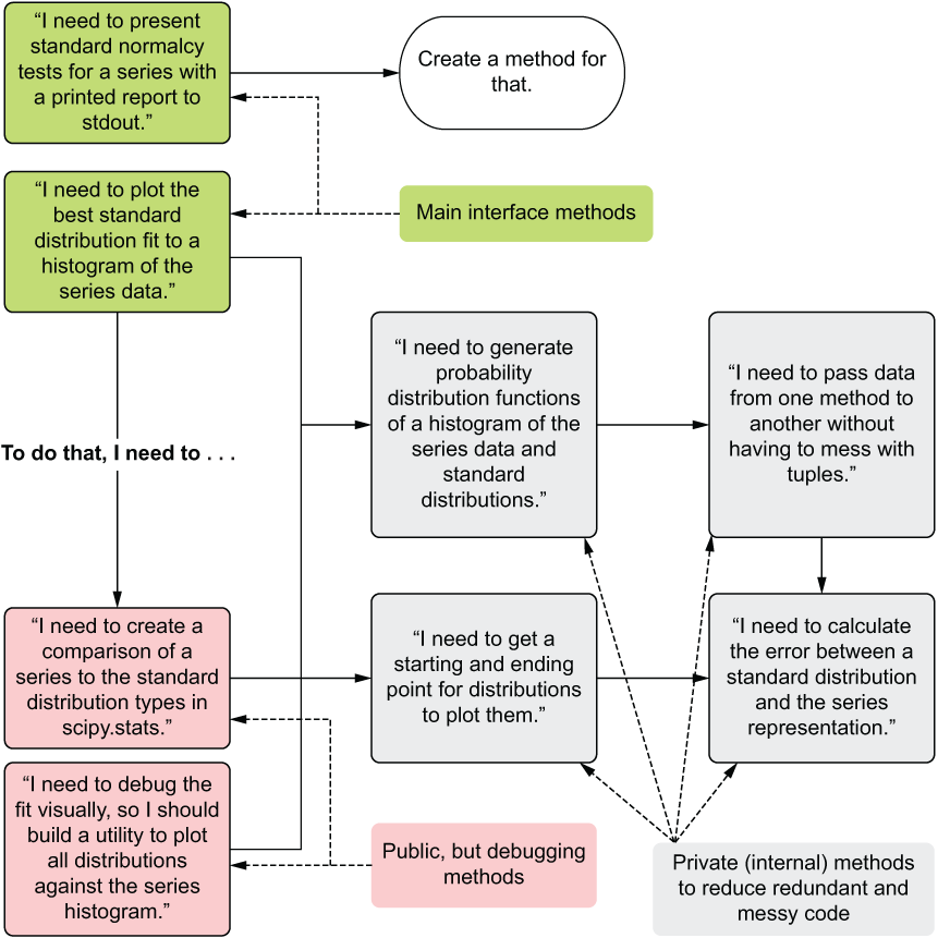
Figure 9.6 The design process for listing 9.3, focusing on testability and isolable code structure

Each of the boxes to the right of the leftmost column in figure 9.6 represents distinct logical operations that have been separated out for the purposes of testing. Breaking up the components in this way enables us to have fewer places that we have to search through. We also reduce the code complexity by isolating individual functionality, making a complicated series of actions little more than a path of complex actions, each stage capable of being checked and validated for proper functionality independent of one another.

NOTE While writing these examples, I actually wrote listing 9.3 first, and then later adapted listing 9.1 from that code. Writing from the perspective of generating unit-testable code from the start helps keep your solutions easier to read, modify, and, of course, test (or, in this case, convert into a hard-to-read script). When getting started in writing abstract code, the process of creating abstraction may seem foreign. As with anything else in this profession, you will naturally gravitate toward more efficient methods over time. Don’t be discouraged if you feel that you are going from script to abstraction in refactoring. Before you know it, you’ll be leaving the world of scripting behind.

To further explain how the thought process in figure 9.6 translates from structural design into creating testable code in succinct and isolable groupings of functionality, let’s take a look at the private method _generate_boundaries() as an example. The following listing shows what a simple unit test for this private method would look like.

Listing 9.4 An example unit test for the _generate_boundaries() method

def test_generate_boundaries():                                           ❶
    expected_low_norm = -2.3263478740408408                               ❷
    expected_high_norm = 2.3263478740408408
    boundary_arguments = {'location': 0, 'scale': 1, 'arguments': ()}
    test_object = DistributionAnalysis(np.arange(0,100), 10)              ❸
    normal_distribution_low = test_object._generate_boundaries(stat.norm, 
                                            boundary_arguments, 
                                            0.01)                         ❹
    normal_distribution_high = test_object._generate_boundaries(stat.norm, 
                                            boundary_arguments, 
                                            0.99)
    assert normal_distribution_low == expected_low_norm, 
      'Normal Dist low boundary: {} does not match expected: {}' 
      .format(normal_distribution_low, expected_low_norm)                 ❺
    assert normal_distribution_high == expected_high_norm, 
      'Normal Dist high boundary: {} does not match expected: {}' 
      .format(normal_distribution_high, expected_high_norm)
 
if __name__ == '__main__':                                                ❻
    test_generate_boundaries()
    print('tests passed')

❶ A unit test definition function for testing the _generate_boundaries() method

❷ Static test values that we’re expecting as a result to ensure proper functionality

❸ Object instantiation of our class DistributionAnalysis()

❹ Calls the protected method _generate_boundaries with the lower boundary value of 0.01

❺ Asserts that the return from the _generate_boundaries method equals our expected value

❻ Allows for all tests for the module to be run (in practice, multiple unit test functions will be called here). If all tests pass (assertions don’t throw assertion exceptions), this script will exit, printing that tests passed.

In this approach, we’re testing several conditions to ensure that our method works as we expect. It’s important to note from this example that, if this block of code were not isolated from the remainder of the actions going on in this module, it would be incredibly challenging (or impossible) to test. If this portion of the code was causing a problem (if one arose) or another tightly coupled action that preceded or followed this code, we wouldn’t have any way of determining the culprit without modifying the code. However, by separating out this functionality, we can test at this boundary and determine whether it is behaving correctly, thereby reducing the number of things we need to evaluate if the module does not do what it is intended to do.

Note Many Python unit-test frameworks exist, each with its own interface and behavior (pytest, for instance, relies heavily on fixture annotations). JVM-based languages generally rely on standards set by xUnit, which look dramatically different from those in Python. The point here is not to use one particular style, but rather to write code that is testable and stick to a particular standard of testing.

To demonstrate what this paradigm will do for us in practice, let’s see what happens when we switch the second assertion statement from equality to non-equality. When we run this test suite, we get the following output as an AssertionError, detailing exactly what (and where) things went wrong with our code.

Listing 9.5 An intentional unit-test failure

=================================== FAILURES ===================================
___________________________ test_generate_boundaries ___________________________
 
    def test_generate_boundaries():
        expected_low_norm = -2.3263478740408408
        expected_high_norm = 2.3263478740408408
        boundary_arguments = {'location': 0, 'scale': 1, 'arguments': ()}
        test_object = DistributionAnalysis(np.arange(0, 100), 10)
        normal_distribution_low = test_object._generate_boundaries(stat.norm,
                                                                   boundary_arguments,
                                                                   0.01)
        normal_distribution_high = test_object._generate_boundaries(stat.norm,
                                                                    boundary_arguments,
                                                                    0.99)
        assert normal_distribution_low == expected_low_norm, 
            'Normal Dist low boundary: {} does not match expected: {}' 
                .format(normal_distribution_low, expected_low_norm)
>       assert normal_distribution_high != expected_high_norm,                     ❶
            'Normal Dist high boundary: {} does not match expected: {}' 
                .format(normal_distribution_high, expected_high_norm)
E       AssertionError: Normal Dist high boundary: 2.3263478740408408 does not match expected: 2.3263478740408408                                           ❷
E       assert 2.3263478740408408 != 2.3263478740408408                             ❸
 
ch09/UnitTestExample.py:20: AssertionError
=========================== 1 failed in 0.99 seconds ===========================
Process finished with exit code 0

❶ The caret at the edge of this report shows the line in our unit test that failed.

❷ The return of the top-level exception (the AssertionError) and the message that we put within the test to ensure we can track down what went wrong

❸ The actual evaluation that the assertion attempted to perform

Designing, writing, and running effective unit tests is absolutely critical for production stability, particularly when thinking of future code refactoring or extending the functionality of this utility module, since additional work may change the way that this method or others that feed data into this module function. We do, however, want to know before we merge code into the master (or main) branch that the changes being made will not introduce issues to the rest of the methods in this module (as well as giving us direct insight into where a problem may lie since the functionality is isolated from other code in the module). By having this security blanket of knowing that things work as originally intended, we can confidently maintain complex (and hopefully not complicated) code bases.

NOTE For more information on TDD, I highly encourage you to check out Kent Beck’s book, Test-Driven Development by Example (Addison-Wesley Professional, 2002).

Summary

• Monolithic scripts are not only difficult to read but also force inefficient and error-prone debugging techniques.
• Large, eagerly evaluated scripts are incredibly challenging in terms of modifying behavior and introducing new features. Troubleshooting failures in these becomes an exercise in frustration.
• Defining logical separation of tasks by using abstraction within an ML code base greatly aids legibility for other team members who will need to maintain and improve a solution over time.
• Designing project code architecture to support discrete testable interfaces to functionality greatly helps in debugging, feature enhancement work, and continued maintenance updates to long-lived ML projects.