
3. Editing Worksheets
Editing Worksheets
Microsoft Excel offers a number of features and techniques that you can use to modify your worksheets.
• Use standard editing techniques and the Clear command to change or clear the contents of cells.
• Use Cells group commands to insert or delete cells, columns, and rows.
• Use Clipboard group commands, the fill handle, and drag-and-drop editing to copy cells from one location to another, including cells containing formulas.
• Use the fill handle and Editing group commands to copy cell contents to multiple cells or create a series.
• Modify formulas so they are properly updated by Excel when copied.
• Use Clipboard group commands and drag-and-drop editing to move cells from one location to another.
• Undo and redo multiple actions.
This chapter covers all of these techniques.
Editing Cell Contents
You can use standard editing techniques to edit the contents of cells either as you enter values or formulas or after you have completed an entry. You can also clear a cell’s contents, leaving the cell empty.
To edit as you enter
1. If necessary, click to position the blinking insertion point cursor in the cell (Figure 1) or formula bar (Figure 2).
Figure 1. To edit a cell’s contents while entering information, click to reposition the insertion point in the cell ...

Figure 2. ... or in the formula bar and make changes as desired.
![]()
2. Press ![]() to delete the character to the left of the insertion point.
to delete the character to the left of the insertion point.
or
Type the characters that you want to insert at the insertion point.
To edit a completed entry
1. Double-click the cell containing the incorrect entry to activate it for editing.
2. If the cell contains a value, follow the instructions in the previous section to insert or delete characters as desired.
or
If the cell contains a formula, color-coded Range Finder frames graphically identify cell references (Figures 3 and 5). There are three ways to edit cell references:
• Edit the reference as discussed in the previous section.
• Drag a frame border to move the frame over another cell. As shown in Figure 4, the mouse pointer looks like an arrow as you drag.
• Drag a frame handle to expand or contract it so the frame includes more or fewer cells. As shown in Figure 6, the mouse pointer turns into a two-headed arrow when you position it on a frame handle and drag.
Figure 3. The range Finder frames clearly indicate the problem with this formula.
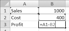
Figure 4. You can drag a Range Finder frame to correct the cell reference. In this example, the Range Finder frame on cell A1 is dragged to cell B1.
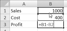
Figure 5. In this example, the Range Finder indicates that the range of cells in the formula excludes a cell.

Figure 6. You can drag a Range Finder frame handle to expand the range and correct the reference in the formula.
To clear cell contents
1. Select the cell(s) you want to clear.
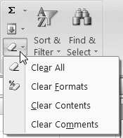
2. Choose Home > Editing > Clear > Clear Contents (Figure 7).
Figure 7. Use options under the Clear menu in the Editing group to remove cell contents or formatting.
or
Press ![]() .
.
• Another way to clear the contents of just one cell is to select the cell, press ![]() , and then press
, and then press ![]() .
.
• Do not press ![]() to clear a cell’s contents! Doing so inserts a space character into the cell. Although the contents seem to disappear, they are just replaced by an invisible character.
to clear a cell’s contents! Doing so inserts a space character into the cell. Although the contents seem to disappear, they are just replaced by an invisible character.
• Clearing a cell is very different from deleting a cell. When you clear a cell, the cell remains in the worksheet—only its contents are removed. When you delete a cell, the entire cell is removed from the worksheet and other cells shift to fill the gap. I tell you about inserting and deleting cells next.
• The Clear Contents command clears only the values or formulas entered into a cell. The other Clear menu commands (Figure 7) work as follows:
• Clear All clears everything, including formatting and comments.
• Clear Formats clears only cell formatting.
• Clear Comments clears only cell comments.
I tell you about formatting cells in Chapter 6 and about adding cell comments in Chapter 11.
Inserting & Deleting Cells
Commands in Excel’s Insert and Delete menus enable you to insert and delete columns, rows, or cells.
• When you insert cells, Excel shifts cells down or to the right to make room for the new cells.
• When you delete cells, Excel shifts cells up or to the left to fill the gap left by the missing cells.
Figures 9, 11, 13, and 15 show examples of how inserting a column or deleting a row in a simple worksheet (Figure 8) affects the cells in a worksheet. Fortunately, Excel is smart enough to adjust cell references in formulas so the formulas you write remain correct.
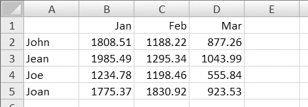
To insert a column or row
1. Select a column or row (Figure 9).
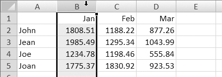
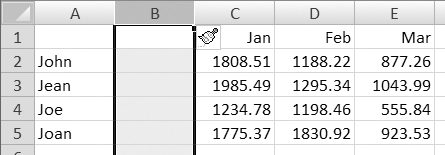
2. Click Home > Cells > Insert or choose an option from the Insert menu (Figure 10). The column or row is inserted and the Insert Options button appears (Figure 11).
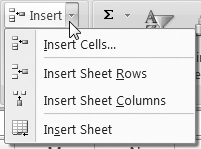
Figure 11. An inserted column.
3. If desired, choose a formatting option for the inserted column or row from the Insert Options pop-up menu (Figure 12).
Figure 12. You can use the Insert Options pop-up menu to set formatting options for inserted cells.

• To insert multiple columns or rows, in step 1, select the number of columns or rows you want to insert. For example, if you want to insert three columns before column B, select columns B, C, and D.
To delete a column or row
1. Select a column or row (Figure 13).

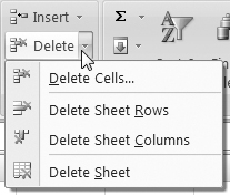
2. Click Home > Cells > Delete or choose an option from the Delete menu (Figure 14).
The column or row (Figure 15)—along with all of its contents—disappears.
Figure 15. The row selected in Figure 13 is deleted.

• To delete more than one column or row at a time, in step 1, select all of the columns or rows you want to delete.
• If you delete a column or row that contains referenced cells, the formulas that reference the cells may display a #REF! error message (Figure 16). This means that Excel can’t find a referenced cell. If this happens, you’ll have to rewrite any formulas in cells displaying the error.
Figure 16. In this example, I deleted a row containing a value referenced in the formula in B6. Because Excel can’t find one of the references it needs, it displays a #REF! error.

To insert cells
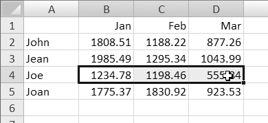
1. Select a cell or range of cells (Figure 17).
Figure 17. Selecting a range of cells.
2. Choose Home > Cells > Insert > Insert Cells (Figure 10).
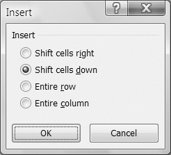
3. In the Insert dialog that appears (Figure 18), select the appropriate option to tell Excel how to shift the selected cells to make room for new cells—Shift cells right or Shift cells down.
4. Click OK. The cells are inserted and the Insert Options button appears (Figure 19).
Figure 19. Here’s what happens when you insert cells selected in Figure 17, using the Shift cells down option.

5. If desired, choose a formatting option for the inserted column or row from the Insert Options pop-up menu.
• Excel always inserts the number of cells that is selected when you use the Insert command (Figures 17 and 19).
To delete cells
1. Select a cell or range of cells to delete (Figure 17).
2. Click Home > Cells > Delete > Delete Cells (Figure 14).
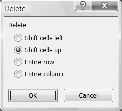
3. In the Delete dialog that appears (Figure 20), select the appropriate option to tell Excel how to shift the other cells when the selected cells are deleted—Shift cells left or Shift cells up.
4. Click OK.
The cells are deleted (Figure 21).
Figure 21. Here’s what happens when you delete the cells selected in Figure 17, using the Shift cells up option.

• If you delete a referenced cell, the formulas that reference the cell may display a #REF! error message (Figure 16). If this happens, you’ll have to rewrite formulas in cells displaying the error.
Copying Cells
Excel offers several ways to copy the contents of one cell to another: the Copy and Paste commands, the fill handle, and the Fill menu command.
How Excel copies depends not only on the method used, but on the contents of the cell(s) being copied.
• When you use the Copy and Paste commands to copy a cell containing a value, Excel makes an exact copy of the cell, including any formatting (Figure 22). I tell you about formatting cells in Chapter 6.
Figure 22. The Copy and Paste commands can make an exact copy.
• When you use the fill handle or a Fill menu command to copy a cell containing a value, Excel either makes an exact copy of the cell, including any formatting, or creates a series based on the original cell’s contents (Figure 23).
Figure 23. Using the fill handle on a cell containing the word Monday generates a list of the days of the week.

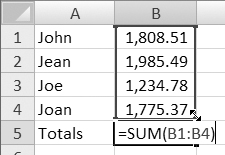
• When you copy a cell containing a formula, Excel copies the formula, changing any relative references in the formula so they’re relative to the destination cell(s) (Figure 24).
Figure 24. Copying a formula that totals a column automatically writes correctly referenced formulas to total similar columns.

Copy & Paste
The Copy and Paste commands in Excel work very much the way they do in other programs. Begin by selecting the source cells and copying them to the Clipboard. Then select the destination cells and paste the Clipboard contents in.
To copy with Copy & Paste
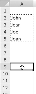
1. Select the cell(s) you want to copy (Figure 25).
Figure 25. Begin by selecting the cell(s) you want to copy.
2. Click Home > Clipboard > Copy (Figure 26) or press ![]() . An animated marquee appears around the selection (Figure 27).
. An animated marquee appears around the selection (Figure 27).
Figure 26. The Clipboard group includes the Paste button/menu and the Cut, Copy, and Format Painter buttons.
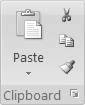
Figure 27. A marquee appears around the selection when it has been copied to the Clipboard.

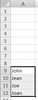
3. Select the cell(s) in which you want to paste the selection (Figure 28). If more than one cell has been copied, you can select either the first cell of the destination range or the entire range.
Figure 28. Select the destination cell(s).

4. Click Home > Clipboard > Paste (Figure 26) or press ![]() or
or ![]() . The originally selected cells are copied to the new location and the Paste Options button appears (Figure 29).
. The originally selected cells are copied to the new location and the Paste Options button appears (Figure 29).
Figure 29. The contents of the copied cells appear in the destination cells.

5. If desired, choose an option for the pasted cell(s) from the Paste Options pop-up menu (Figure 30).
Figure 30. You can set formatting for pasted in cells by choosing an option from the Paste Options pop-up menu.

• If the destination cells contain information, Excel may overwrite them without warning you.
• If you click the Paste button or press ![]() , the marquee remains around the copied range, indicating that it is still in the Clipboard and may be pasted elsewhere. The marquee disappears automatically as you work, but if you want to remove it manually, press
, the marquee remains around the copied range, indicating that it is still in the Clipboard and may be pasted elsewhere. The marquee disappears automatically as you work, but if you want to remove it manually, press ![]() .
.
• The Paste Options button will not appear if you press ![]() in step 4.
in step 4.
• The Paste button’s pop-up menu (Figure 31) offers additional options for pasting Clipboard contents. For example, you can convert formulas in the selection into values or paste a cell without border formatting. Choosing Paste Special displays a dialog with even more options (Figure 32).
Figure 31. The Paste button includes a menu of options for pasting Clipboard contents.
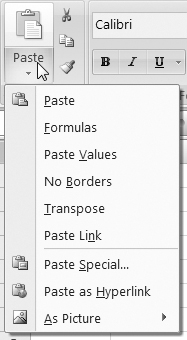
Figure 32. The Paste Special dialog offers additional options for pasting Clipboard contents.

The Fill Handle
The fill handle is a small black or colored box in the lower-right corner of the cell pointer (Figure 33) or selection (Figure 34). You can use the fill handle to copy the contents of one or more cells to adjacent cells.
Figure 33. The fill handle on a single cell.
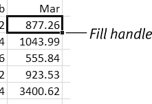
Figure 34. The fill handle on a range of cells.

To copy with the fill handle
1. Select the cell(s) containing the information you want to copy (Figure 34).
2. Position the mouse pointer on the fill handle. The mouse pointer turns into a black plus sign (Figure 35).
Figure 35. When the mouse pointer is over the fill handle, it turns into a black plus sign.
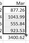
3. Press the mouse button down and drag to the adjacent cells. A gray border surrounds the source and destination cells (Figure 36).
Figure 36. As you drag the fill handle, a gray border indicates the source and destination cell(s).
4. When all the destination cells are surrounded by the gray border, release the mouse button. The cells are filled and the Fill Options button appears (Figure 37).
Figure 37. The destination cells fill with the contents of the source cells.

5. If desired, choose an option for the filled cell(s) from the Fill Options pop-up menu (Figure 38).
Figure 38. Use the Fill Options pop-up menu to set options for the filled in cells.

• You can use the fill handle to copy any number of cells. The destination cells, however, must be adjacent to the original cells.
• When using the fill handle, you can only copy in one direction (up, down, left, or right) at a time.
• If the destination cells contain information, Excel may overwrite them without warning you.
The Fill Commands
The Fill commands work a lot like the fill handle in that they copy information to adjacent cells. But rather than dragging to copy, you select the source and destination cells at the same time and then use a Fill command to complete the copy. The Fill menu in the Home tab’s Editing group (Figure 39) offers several options for copying to adjacent selected cells:
• Down copies the contents of the top cell(s) in the selection to the selected cells beneath it.
• Right copies the contents of the left cell(s) in the selection to the selected cells to the right of it.
• Up copies the contents of the bottom cell(s) in the selection to the selected cells above it.
• Left copies the contents of the right cell(s) in the selection to the selected cells to the left of it.
Figure 39. The Fill menu on the Home tab’s Editing group.

To copy with the Fill command
1. Select the cell(s) you want to copy along with the adjacent destination cell(s) (Figure 40).
Figure 40. To use a Fill command, begin by selecting the source and destination cells.

2. Choose the appropriate command from the Fill menu in the Editing group (Figure 39): Down, Right, Up, Left. The cells are filled as specified (Figure 37).
or
To fill down, press ![]() or to fill right, press
or to fill right, press ![]() .
.
• You must select both the source and destination cells when using a Fill command. If you select just the destination cells, Excel won’t copy the correct cells.
Series & AutoFill
A series is a sequence of cells that forms a logical progression. Excel’s AutoFill feature can generate a series of numbers, months, days, dates, and quarters.
To create a series with the fill handle
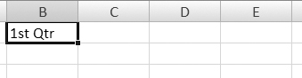
1. Enter the first item of the series in a cell (Figure 41). Be sure to complete the entry by pressing ![]() or clicking the Enter button on the formula bar.
or clicking the Enter button on the formula bar.
Figure 41. To create an AutoFill series, start by entering the first value in a cell.
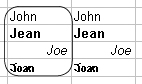
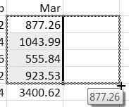
2. Position your mouse pointer on the fill handle and drag. All the cells that will be part of the series are surrounded by a gray border and a yellow box indicates the value that will be in the last cell in the range (Figure 42).
Figure 42. Drag the fill handle to include all cells that will be part of the series.

3. Release the mouse button to complete the series (Figure 43).
Figure 43. Excel creates the series automatically.
To create a series with the Series command
1. Enter the first item of the series in a cell (Figure 41).
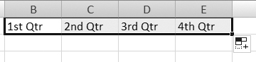
2. Select all cells that will be part of the series, including the first cell (Figure 44).
Figure 44. To use the Series command, select the source and destination cells.

3. Choose Home > Editing > Fill > Series (Figure 39).
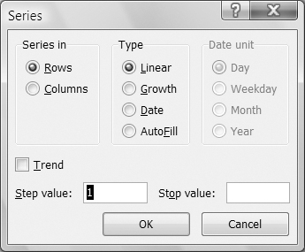
4. In the Series dialog that appears (Figure 45), select the AutoFill option.
Figure 45. Select the AutoFill option in the Series dialog.
5. Click OK to complete the series (Figure 43).
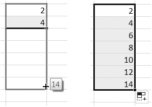
• To generate a series that skips values, enter the first two values of the series in adjoining cells, then use the fill handle or Series command to create the series, including both cells as part of the source (Figures 46 and 47).
Figures 46 & 47. Enter the first two values in the series, then select both cells and drag the fill handle (left) to complete the series (right).
Copying Formulas
You copy a cell containing a formula the same way you copy any other cell in Excel: with the Copy and Paste commands, with the fill handle, or with a Fill command. These methods are discussed earlier in this chapter.
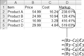
Generally speaking, Excel does not make an exact copy of a formula. Instead, it copies the formula based on the kinds of references used within it. If relative references are used, Excel changes them based on the location of the destination cell in relation to the source cell. You can see an example of this in Figures 48 and 49.
Figure 48. Here’s a formula to calculate markup percentage. If the company has 763 products, would you want to write the same basic formula 762 more times? Of course not!

Figure 49. Copying formulas can save time. If the original formula is properly written, the results of the copied formula should also be correct.
• You’ll find it much quicker to copy formulas rather than to write each and every formula from scratch.
• Not all formulas can be copied with accurate results. For example, you can’t copy a formula that sums up a column of numbers to a cell that should represent a sum of cells in a row (Figure 50).
Figure 50. In this illustration, the formula in cell C11 was copied to cell F7. This doesn’t work because the two cells don’t add up similar ranges. The formula in cell F7 would have to be rewritten from scratch. It could then be copied to F8 through F10. (I tell you about the SUM function in Chapter 5.)

• I explain the various types of cell references—relative, absolute, and mixed—beginning on the next page.
Relative vs. Absolute Cell References
There are two primary types of cell references:
• A relative cell reference is the address of a cell relative to the cell the reference is in. For example, a reference to cell B1 in cell B3, tells Excel to look at the cell two cells above B3. Most of the references you use in Excel are relative references.
• An absolute cell reference is the exact location of a cell. To indicate an absolute reference, enter a dollar sign ($) in front of the column letter(s) and row number(s) of the reference. An absolute reference to cell B1, for example, would be written $B$1.
As Figures 51 and 52 illustrate, relative cell references change when you copy them to other cells. Although in many cases, you might want the references to change, sometimes you don’t. That’s when you use absolute references (Figures 53 and 54).
Figure 51. This formula correctly calculates a partner’s share of profit.
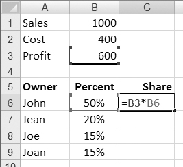
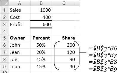
Figure 52. But when the formula is copied for the other partners, the relative reference to cell B3 is changed, causing incorrect results and an error message!

Figure 53. Rewrite the original formula so it includes an absolute reference to cell B3, which all of the formulas must reference.

Figure 54. When the formula is copied for the other partners, only the relative reference (to the percentages) changes. The results are correct.
• Here’s a trick for remembering the meaning of the notation for absolute cell references: in your mind, replace the dollar sign with the word always. Then you’ll read $B$1 as always B always 1—always B1!
• If you’re having trouble understanding how these two kinds of references work and differ, don’t worry. This is one of the most difficult spreadsheet concepts you’ll encounter. Try creating a worksheet like the one illustrated on this page and working your way through the figures one at a time. Pay close attention to how Excel copies the formulas you write!
To include an absolute cell reference in a formula
1. Enter the formula by typing or clicking as discussed in Chapter 2.
2. Insert a dollar sign before the column and row references for the cell reference you want to make absolute (Figure 55).
Figure 55. Type in the dollar signs as needed when you enter an absolute cell reference.

3. Complete the entry by pressing ![]() or clicking the Enter button on the formula bar.
or clicking the Enter button on the formula bar.
• You can edit an existing formula to include absolute references by inserting dollar signs where needed. I tell you how to edit cell contents earlier in this chapter.
• Do not use a dollar sign in a formula to indicate currency formatting. I tell you how to apply formatting to cell contents, including currency format, in Chapter 6.
Mixed References
Once you’ve mastered the concept of relative vs. absolute cell references, consider another type of reference: a mixed cell reference.
In a mixed cell reference, either the column or row reference is absolute while the other reference remains relative. Thus, you can use cell references like A$1 or $A1. Use this when a column reference must remain constant but a row reference changes or vice versa. Figure 56 shows a good example.
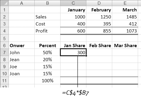
Figure 56. The formula in cell C7 includes two different kinds of mixed references. It can be copied to cells C8 through C10 and C7 through E10 for correct results in all cells. Try it and see for yourself!
Moving Cells
Excel offers two ways to move the contents of one cell to another: the Cut and Paste commands and dragging the border of a selection. Either way, Excel moves the contents of the cell.
• When you move a cell, Excel searches the worksheet for any cells that contain references to it and changes the references to reflect the cell’s new location (Figures 57 and 58).
Figure 57. Note the formula in cell C6.

Figure 58. See how it changes when one of the cells it references moves?

To move with Cut & Paste
1. Select the cell(s) you want to move (Figure 59).
Figure 59. Select the cell(s).
2. Click Home > Clipboard > Cut (Figure 26) or press ![]() . An animated marquee appears around the selection (Figure 60).
. An animated marquee appears around the selection (Figure 60).
Figure 60. When you use the Cut command, a marquee appears around the selection but the selected cells do not disappear.

3. Select the cell(s) in which you want to paste the selection (Figure 61).
Figure 61. Select the destination cell(s).
4. Click Home > Clipboard > Paste (Figure 26) or press ![]() or
or ![]() . The cell contents are moved to the new location (Figure 62).
. The cell contents are moved to the new location (Figure 62).
Figure 62. When you use the Paste command, the selection moves.
• Consult the tips beneath the section titled “To copy with Copy & Paste” for Paste command warnings and tips.
To move with drag & drop
1. Select the cell(s) you want to move (Figure 59).
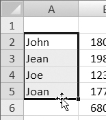
2. Position the mouse pointer on the border of the selection. A four-headed arrow appears beneath the mouse pointer (Figure 63).
Figure 63. When you move the mouse pointer onto the border of a selection, a four-headed arrow appears beneath it.
3. Press the mouse button down and drag toward the new location. As you move the mouse, a gray border the same shape as the selection moves along with it and a box indicates the range where the cells will move (Figure 64).
Figure 64. As you drag, a gray border moves along with the mouse pointer.

4. Release the mouse button. The selection moves to its new location (Figure 62).
• If you try to drag a selection to cells already containing information, Excel warns you with a dialog like the one in Figure 65. If you click OK to complete the move, the destination cells will be overwritten with the contents of the cells you are moving.
Figure 65. Excel warns you when you will overwrite cells with a selection you drag.

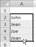
• To copy using drag and drop, hold down ![]() as you press the mouse button down. The mouse pointer turns into an arrow with a tiny plus sign (+) beside it (Figure 66). When you release the mouse button, the selection is copied.
as you press the mouse button down. The mouse pointer turns into an arrow with a tiny plus sign (+) beside it (Figure 66). When you release the mouse button, the selection is copied.
Figure 66. Hold down ![]() to copy a selection by dragging it. A plus sign appears beside the mouse pointer.
to copy a selection by dragging it. A plus sign appears beside the mouse pointer.
• To move and insert cells using drag and drop, hold down ![]() as you press the mouse button down. As you drag, a gray bar moves along with the mouse pointer and a yellow box indicates where the cells will be inserted (Figure 67). When you release the mouse button, the cells are inserted (Figure 68).
as you press the mouse button down. As you drag, a gray bar moves along with the mouse pointer and a yellow box indicates where the cells will be inserted (Figure 67). When you release the mouse button, the cells are inserted (Figure 68).
Figure 67. Hold down ![]() while dragging to insert a selection between other cells. A bar indicates where the cells will be inserted.
while dragging to insert a selection between other cells. A bar indicates where the cells will be inserted.
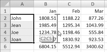
Figure 68. This makes it possible to rearrange the cells in a worksheet.

The Office Clipboard
The Office Clipboard enables you to “collect and paste” multiple items. You simply display the Office Clipboard task pane, then copy text or objects as usual. But instead of the Clipboard contents being replaced each time you use the Copy or Cut command, all items are stored on the Office Clipboard (Figure 69). You can then paste any of the items on the Office Clipboard into your Excel document.
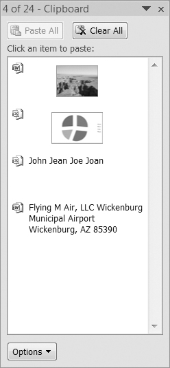
Figure 69. The Clipboard task pane with four items: a picture from Word, an Excel chart, some Excel worksheet cells, and some text from Word.
• The Office Clipboard works with all Microsoft Office applications—not just Excel—so you can store items from different types of Office documents.
• This feature was referred to as Collect and Paste in previous versions of Microsoft Office for Windows.
To display the Office Clipboard
Click the Dialog Box Launcher button in the bottom-right corner of the Home tab’s Clipboard group (Figure 26). The Office Clipboard appears as a task pane beside the document window (Figure 70).
Figure 70. The Office Clipboard appears as a task pane.

To add an item to the Office Clipboard
1. If necessary, display the Office Clipboard (Figure 70).
2. Select the cells or object you want to copy (Figure 59).
3. Click Home > Clipboard > Copy (Figure 26) or press ![]() . The selection appears on the Office Clipboard (Figure 71).
. The selection appears on the Office Clipboard (Figure 71).
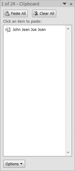
Figure 71. The cells you selected are added to the Clipboard.
To use Office Clipboard items
1. If necessary, display the Office Clipboard.
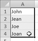
2. In the document window, select the top-left cell where you want to paste the Office Clipboard item (Figure 72).
Figure 72. Select the top-left cell where you want to paste the item.

3. In the Office Clipboard task pane, click the item you want to paste into the document (Figure 73).
Figure 73. When you point to or click an item, a border appears around it.

Or
1. If necessary, display the Office Clipboard.
2. Drag the item you want to use from the Office Clipboard into the document window.
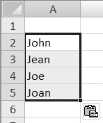
The item you pasted or dragged appears in the document window (Figure 74).
Figure 74. The item you pasted appears in the document.
• Not all items can be pasted into worksheet cells. Graphics, for example, are pasted on top of the worksheet layer. Graphic objects are covered in Chapter 7.
To remove Office Clipboard items
1. In the Office Clipboard window, point to the item you want to remove (Figure 73). A blue border appears around it and a pop-up menu button appears beside it.
2. Click the pop-up menu button to display a menu of two options (Figure 75).
Figure 75. You can access a pop-up menu like this one for each item on the Office Clipboard.

3. Choose Delete. The item is removed from the Office Clipboard (Figure 76).
Figure 76. Choosing Delete for an item removes it from the Office Clipboard.

Or
Click the Clear All button at the top of the Office Clipboard (Figure 69) to remove all items.
Undoing & Redoing Actions
Excel’s Quick Access toolbar (Figure 77) offers buttons and menus that enable you to undo or redo the last things you did.
Figure 77. The Undo and Redo buttons on the Quick Access toolbar.

• Undo reverses your last action. Excel supports multiple levels of undo, enabling you to reverse more than just the very last action.
• Redo reverses the Undo command. This command is only available if the last thing you did was use the Undo command.
• Think of the Undo command as the Oops command—anytime you say “Oops,” you’ll probably want to use it.
To undo the last action
Click the Undo button (Figure 77) or press ![]() .
.
To undo multiple actions
Click the Undo button (Figure 77) or press ![]() repeatedly.
repeatedly.
Or
1. Click the triangle beside the Undo button to display a pop-up menu of recent actions.
2. Drag down to select all the actions that you want to undo (Figure 78).
Figure 78. Use the Undo button’s menu to select multiple actions to undo.
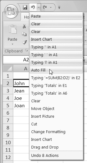
3. Release the mouse button to undo all selected actions.
To reverse the last undo
Click the Redo button (Figure 77) or press ![]() .
.
To reverse multiple undos
Click the Redo button (Figure 77) or press ![]() repeatedly.
repeatedly.
Or
1. Click the triangle beside the Redo button on the Standard toolbar to display a drop-down list of recently undone actions.
2. Drag down to select all the actions that you want to redo (Figure 79).
Figure 79. You can also use the Redo button’s menu to select multiple actions to redo.
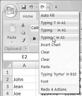
3. Release the mouse button to reverse all selected undos.