
13. Advanced Techniques
Advanced Techniques
Microsoft Excel has many advanced features that you can use to tap into Excel’s real power. In this chapter, I tell you about some of the advanced techniques I think you’ll find most useful in your day-to-day work with Excel:
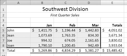
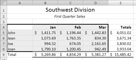
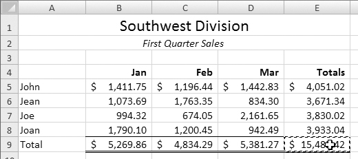
• Names (Figure 1) let you assign easy-to-remember names to cell references. You can then use the names in place of cell references in formulas.
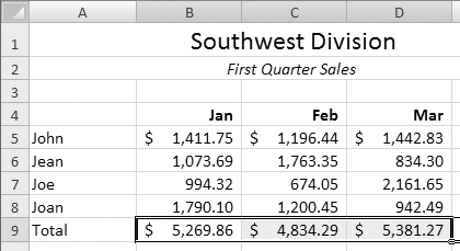
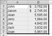
Figure 1. The reference to the selected range would be a lot easier to remember if it had a name like FirstQtrSales rather than just A5:D8.
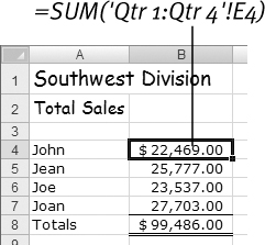
• 3-D cell references (Figure 2) let you write formulas with links to other worksheets and workbooks.
Figure 2. 3-D cell references make it possible to link information between worksheets or workbooks.
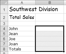
• Consolidations (Figure 3) let you summarize information from several source areas into one destination area.
Figure 3. Excel’s consolidation feature lets you combine information from multiple source areas into one destination area—with or without live links.

• Custom views enable you to create predefined views of workbook contents that can include a variety of settings.
• Macros let you automate repetitive tasks and build custom Excel-based applications.
• This chapter builds on information in previous chapters. It’s a good idea to have a solid understanding of the information covered up to this point in this book before exploring the features in this chapter.
Names
The trouble with using cell references in formulas is that they’re difficult to remember. To make matters worse, cell references can change if cells above or to the left of them are inserted or deleted.
Excel’s Names feature eliminates both problems by letting you assign easy-to-remember names to individual cells or ranges of cells in your workbooks. The names, which you can use in formulas, don’t change, no matter how much worksheet editing you do.
• Excel can automatically recognize many column and row labels as cell or range names. I tell you about this feature on the next page.
• Names can be up to 255 characters long and can include letters, numbers, periods, question marks, and underscore characters (_). The first character must be a letter. Names cannot contain spaces or “look” like cell references.
• If you enter an incorrect name reference in a formula, a #NAME? error value appears in the cell (Figure 4).
Figure 4. If a name reference in a formula is not correct, a #NAME? error appears in the cell.

To define a name
1. Select the cell(s) you want to name (Figure 1).
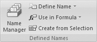
2. Choose Formulas > Defined Names > Define Name (Figure 5).
Figure 5. The Defined Names group offers a number of options for working with names.
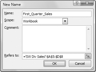
3. In the New Name dialog that appears, Excel may suggest a name in the text box. You can enter a name you prefer (Figure 6).
Figure 6. Use the New Name dialog to set a name for one or more cells. As you can see, the name of the worksheet is part of the cell reference.
4. Choose an option from the Scope drop-down list to indicate whether the name should be valid in the entire workbook file or just one of its sheets.
5. If desired enter a comment for the name in the Comment box.
6. The cell reference in the Refers to text box should reflect the range you selected in step 1. To enter a different range, delete the range that appears in the text box and either type in a new range or reselect the cell(s) in the worksheet window.
7. Click OK.
• Previous versions of Excel enabled you to use column and row headings as labels. That feature is no longer supported in Excel 2007.
To create names
1. Select the cells containing the ranges you want to name as well as text in adjoining cells that you want to use as names (Figure 7).
Figure 7. To use the Create Names dialog, you must first select the cells you want to name, as well as adjoining cells with text you want to use as names.
2. Choose Formulas > Defined Names > Create from Selection (Figure 5).
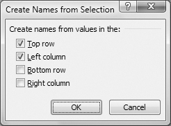
3. In the Create Names from Selection dialog (Figure 8), turn on the check box(es) for the cells that contain the text you want to use as names.
Figure 8. In the Create Names from Selection dialog, tell Excel which cells contain the text for names.
4. Click OK.
Excel uses the text in the cells you indicated as names for the adjoining cells. You can see the results if you open the Name Manager dialog (Figure 9).
Figure 9. Look in the Name Manager dialog to see how many names were added and to remove names.

To modify or delete a name
1. Click Formulas > Defined Names > Name Manager (Figure 5).
2. In the Name Manager dialog (Figure 9), click to select the name in the scrolling list that you want to modify or delete.
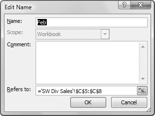
3. To modify the name, click Edit. Then use the Edit Name dialog (Figure 10) to modify the name’s settings and click OK.
Figure 10. Use the Edit name dialog to change settings for a name.
or
To delete the name, click Delete. The name disappears.
4. Repeat steps 2 and 3 to modify or delete other names as desired.
5. Click the Close button to dismiss the Name Manager dialog.
To enter a name in a formula
1. Select the cell in which you want to write the formula.
2. Type in the formula, replacing any cell reference with the corresponding name (Figure 11).
Figure 11. Once a range has been named, it can be used instead of a cell reference in a formula.

3. Press ![]() or click the Enter button the formula bar.
or click the Enter button the formula bar.
Excel performs the calculation just as if you’d typed in a cell reference (Figure 12).
Figure 12. When you complete the formula, the result appears in the cell.

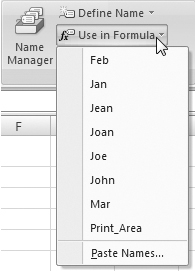
• You can use the Use in Formula menu’s options to paste a name into a formula for you. Follow the steps above, but when it’s time to type in the name, click Formulas > Defined Names > Use in Formula to display a menu of defined names (Figure 13). Then choose the name you want to paste in. The Use in Formula menu even works when you use the Function Arguments dialog to write formulas. I tell you about the Function Arguments dialog in Chapter 5.
Figure 13. You can paste in a name by choosing it from the Use in Formula menu.
• When you delete a name, Excel responds with a #NAME? error in each cell that contains a formula referring to that name (Figure 4). These formulas must be rewritten.
To apply names to existing formulas
1. Select the cells containing formulas for which you want to apply names. If you want to apply names throughout the worksheet, click any single cell.
2. Choose Formulas > Defined Names > Define Name > Apply Names (Figure 14).
Figure 14. Choose Apply Names from the Define Name menu.

3. In the Apply Names dialog (Figure 15), select the names that you want to use in place of the cell reference. To select or deselect a name, click on it.
Figure 15. Select the names that you want to apply to formulas in your worksheet.

4. Click OK.
Excel rewrites the formulas with the appropriate names from those you selected. Figure 16 shows an example of formulas changed by selecting Jan, Feb, and Mar in Figure 15.
Figure 16. Excel applies the names you selected to formulas that reference their ranges.
• If only one cell is selected, Excel applies names based on your selection(s) in the Apply Names dialog instead of using the selected cell.
• If you turn off the Ignore Relative/Absolute check box in the Apply Names dialog (Figure 15), Excel matches the type of reference. I tell you about relative and absolute references in Chapter 3.
To select named cells
Choose the name of the cell(s) you want to select from the Name drop-down list on the far-left end of the formula bar (Figure 17).
Figure 17. The Name drop-down list on the left end of the formula bar lets you select named ranges quickly.

Or
1. Click the Name box at the far-left end of the formula bar to select it.
2. Type in the name of the cells you want to select (Figure 18).
Figure 18. If you prefer, you can type in a name and press ![]() to select it.
to select it.
![]()
3. Press ![]() .
.
Or
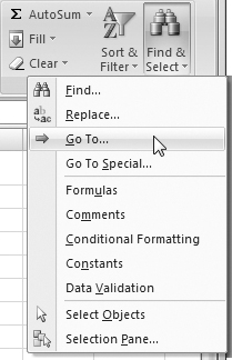
1. Choose Home > Editing > Find & Select > Go To (Figure 19) or press ![]() .
.
Figure 19. Choose the Go To command on the Find & Select menu.
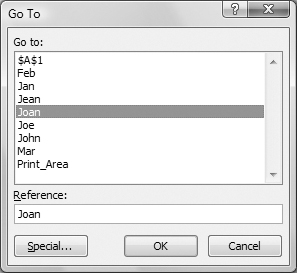
2. In the Go To dialog that appears (Figure 20), click the name of the cell(s) you want to select in the Go to scrolling list.
Figure 20. Select the name of the cell(s) you want to use from the Go to scrolling list.
3. Click OK.
• When named cells are selected, the name appears in the cell reference area at the far-left end of the formula bar.
3-D References
3-D cell references let you write formulas that reference cells in other worksheets or workbooks. The links are live—when a cell’s contents change, the results of formulas in cells that reference it change.
Excel offers several ways to write formulas with 3-D cell references:
• Use cell names. I tell you about cell names in the first part of this chapter. Figure 21 shows an example.
Figure 21. This example uses the SUM function to add the contents of the cells named John, Joan, Joe, and Jean in the same workbook.
![]()
• Type them in. When you type in a 3-D cell reference, you must include the name of the sheet (in single quotes, if the name contains a space), followed by an exclamation point (!) and cell reference. If the reference is for a cell in another workbook, you must also include the workbook name, in brackets. Figures 22, 23, and 24 show examples.
Figure 22. This example refers to cell B9 in a worksheet called Results for Year in the same workbook.
![]()
Figure 23. This example uses the SUM function to add the contents of cell E9 in worksheets starting with Qtr 1 and ending with Qtr 4 in the same workbook.
![]()
Figure 24. This example refers to cell B9 in a worksheet called Results for Year in a workbook called Sales.xlsx.
![]()
• Click on them. You’ll get the same results as if you had typed the references, but Excel does all the typing for you. (This is the method I prefer.)
• Use the Paste Link command. This command lets you paste a link between cells in different sheets of a workbook or different workbooks.
• When you delete a cell, Excel displays a #REF! error in any cells that referred to it. The cells containing these errors must be revised to remove the error.
• Do not make references to an unsaved file. If you do and you close the file with the reference before saving (and naming) the file it refers to, Excel won’t be able to update the link.
To reference a named cell or range in another worksheet
1. Select the cell in which you want to enter the reference.
2. Type an equal sign (=).
3. If the sheet containing the cells you want to reference is in another workbook, type the name of the workbook (within single quotes, if the name contains a space) followed by an exclamation point (!).
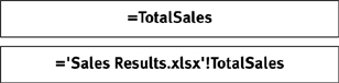
4. Type the name of the cell(s) you want to reference (Figures 25 and 26).
Figures 25 & 26. Two examples of 3-D references utilizing names. The first example refers to a name in the same workbook. The second example refers to a name in a different book. In both instances the scope of the named range is set to workbook.
5. Press ![]() or click the Enter button on the formula bar.
or click the Enter button on the formula bar.
• If the name you want to reference is in the same workbook, you can paste it in by choosing a name from the Use in Formula menu on the Define Names menu (Figure 13). I tell you how to use the Use in Formula menu earlier in this chapter.
To reference a cell or range in another worksheet by clicking
1. Select the cell in which you want to enter the reference.
2. Type an equal sign (=).
3. If the sheet containing the cells you want to reference is in another workbook, switch to that workbook.
4. Click on the sheet tab for the worksheet containing the cell you want to reference.
5. Select the cell(s) you want to reference (Figure 27).
Figure 27. After typing an equal sign in the cell in which you want the reference to go, you can select the cell(s) you want to reference.
6. Press ![]() or click the Enter button on the formula bar.
or click the Enter button on the formula bar.
To reference a cell or range in another worksheet by typing
1. Select the cell in which you want to enter the reference.
2. Type an equal sign (=).
3. If the sheet containing the cells you want to reference is in another workbook, type the name of the workbook within brackets ([]).
4. Type the name of the sheet followed by an exclamation point (!).
5. Type the cell reference for the cell(s) you want to reference.
6. Press ![]() or click the Enter button on the formula bar.
or click the Enter button on the formula bar.
• If the name of the sheet includes a space character, the sheet name must be enclosed within single quotes in the reference. See Figures 22, 23, and 24 for examples.
To reference a cell with the Paste Link command
1. Select the cell you want to reference.
2. Choose Home > Clipboard > Copy (Figure 28) or press ![]() .
.
Figure 28. The Clipboard group.

3. Switch to the worksheet in which you want to put the reference.
4. Select the cell in which you want the reference to go.
5. Choose Home > Clipboard > Paste > Paste Link (Figure 29).
Figure 29. You can use the Paste Link command to paste a link to one cell into another cell.

• Do not press ![]() after using the Paste Link command! Doing so pastes the contents of the Clipboard into the cell, overwriting the link.
after using the Paste Link command! Doing so pastes the contents of the Clipboard into the cell, overwriting the link.
• Using the Paste Link command to paste a range of cells creates a special range called an array. Each cell in an array shares the same cell reference and cannot be changed unless all cells in the array are changed.
To write a formula with 3-D references
1. Select the cell in which you want to enter the formula.
2. Type an equal sign (=).
3. Use any combination of the following techniques until the formula is complete.
• To enter a function, use the Function Arguments dialog or type in the function. I tell you how to use the Function Arguments dialog in Chapter 5.
• To enter an operator, type it in. I tell you about using operators in Chapter 2.
• To enter a cell reference, select the cell(s) you want to reference or type the reference in. If typing the reference, be sure to include single quotes, brackets, and exclamation points as discussed on the previous page.
4. Press ![]() or click the Enter button on the formula bar.
or click the Enter button on the formula bar.
To write a formula that sums the same cell on multiple, adjacent sheets
1. Select the cell in which you want to enter the formula.
2. Type =SUM( (Figure 30).
Figure 30. Type the beginning of a formula with the SUM function ...

3. If the cells you want to add are in another workbook, switch to that workbook.
4. Click the sheet tab for the first worksheet containing the cell you want to sum.
5. Hold down ![]() and click on the sheet tab for the last sheet containing the cell you want to sum. All tabs from the first to the last become selected (Figure 31). The formula in the formula bar should look something like the one in Figure 32.
and click on the sheet tab for the last sheet containing the cell you want to sum. All tabs from the first to the last become selected (Figure 31). The formula in the formula bar should look something like the one in Figure 32.
Figure 31. ... select all of the tabs for sheets that contain the cells you want to sum ...
![]()
Figure 32. ... so the sheet names are appended as a range in the formula bar.
![]()
6. Click the cell you want to sum (Figure 33). The cell reference is added to the formula (Figure 34).
Figure 33. Then click on the cell you want to add ...
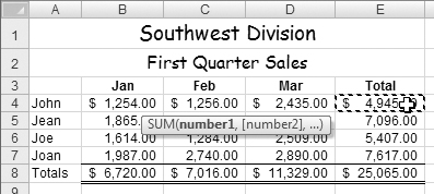
Figure 34. ... so that its reference is appended to the formula in the formula bar.
![]()
7. Type ).
8. Press ![]() or click the Enter button on the formula bar.
or click the Enter button on the formula bar.
• Use this technique to link cells of identically arranged worksheets. This results in a “3-D worksheet” effect.
• Although you can use this technique to consolidate data, the Consolidate command, which I discuss later in this chapter, automates consolidations with or without links.
Opening Workbooks with Links
When you open a workbook that has a link to another workbook file, Excel needs to retrieve the linked information from that file. Whether it does this depends on Excel’s Trust Center settings for external content.
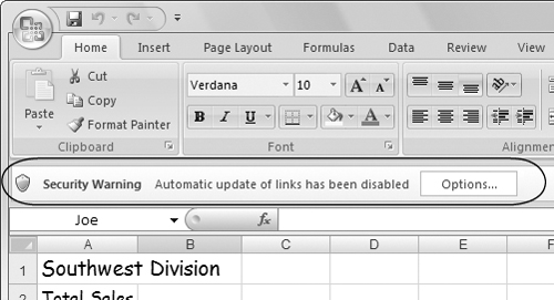
By default, Excel is set to prompt you when Excel needs to retrieve content from another file. It does this by displaying a security warning in the Message Bar between the Ribbon and the Formula bar (Figure 35).
Figure 35. A security warning appears in the message bar when you open a file that contains a link to another file.
In this section, I explain how to allow content to be retrieved and how to modify Trust Center settings for all external links.
• You can also update a link to another file by simply opening the other file. Excel assumes that if the file is secure enough to open, it’s secure enough to retrieve data from.
To allow link updating
1. In the Message Bar’s security warning (Figure 35), click the Options button.
The Microsoft Office Security Options dialog appears (Figure 36).
Figure 36. Use this dialog to set link updating options for a specific workbook file.
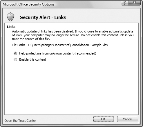
2. Select the Enable this content option.
3. Click OK.
From that point forward, Excel always automatically updates links in the file.
• Links can be used to access information on your computer without your permission. You should not update links in a file if you don’t trust the source of the file, especially if you weren’t expecting the file to include links.
To modify external content settings for links
1. Choose Microsoft Office > Excel Options.
2. In the Excel Options dialog that appears, click the Trust Center item in the list to display Trust Center options (Figure 37).
Figure 37. Click Trust Center in the Excel Options dialog to display Trust Center information and options.

3. Click the Trust Center Settings button.
4. In the Trust Center dialog that appears, click the External Content item in the list to display the External Content options (Figure 38).
Figure 38. Use the Trust Center dialog to set default options for external content such as links.

5. Select one of the Security Settings for Workbook Links options:
• Enable automatic update for all Workbook Links automatically updates links to other files in all workbooks. This disables the security over links.
• Prompt user on automatic update for Workbook Links displays the Security Alert discussed on the previous page when you open a workbook file with links to an unopened workbook file. This is the default setting.
• Disable automatic update of Workbook Links prevents workbook links from being updated automatically. Selecting this option could result in out-of-date information appearing in the workbook.
6. Click OK to save your settings and dismiss the Trust Center dialog.
7. Click OK to dismiss the Excel Options dialog.
• If you often open workbook files created by others, it really isn’t a good idea to enable automatic update for all workbook links. Doing so can create serious security problems.
Consolidations
The Consolidate command lets you combine data from multiple sources. Excel lets you do this in two ways:
• Consolidate based on the arrangement of data. This is useful when data occupies the same number of cells in the same arrangement in multiple locations (Figure 3).
• Consolidate based on identifying labels or categories. This is useful when the arrangement of data varies from one source to the next.
• With either method, Excel can create links to the source information so the consolidation changes automatically when linked data changes.
To consolidate based on the arrangement of data
1. Select the cell(s) where you want the consolidated information to go (Figure 39).
Figure 39. Select the cells in which you want the consolidated data to go.
2. Click Data > Data Tools > Consolidate (Figure 40).
Figure 40. The Data Tools group on the Ribbon’s Data tab.

3. In the Consolidate dialog (Figure 41), choose a function from the Function drop-down list (Figure 42).
Figure 41. Use the Consolidate dialog to identify the cells you want to combine.
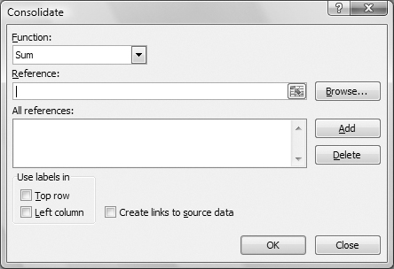
Figure 42. Choose a function for the consolidation from the Function drop-down list.

4. If necessary, click in the Reference box.
5. Switch to the worksheet containing the first cell(s) to be included in the consolidation. The reference is entered into the Reference box.
6. Select the cell(s) you want to include in the consolidation. The reference is entered into the Reference text box (Figure 43).
Figure 43. Enter references for cells in the Consolidate dialog by selecting them in the worksheet.

8. Repeat steps 5, 6, and 7 for all of the cells that you want to include in the consolidation. When you’re finished, the All references scrolling list in the Consolidate dialog might look something like Figure 44.
Figure 44. The cells you want to consolidate are listed in the All references scrolling list in the Consolidate dialog.

9. To create links between the source data and destination cell(s), turn on the Create links to source data check box.
10. Click OK.
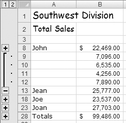
Excel consolidates the information in the originally selected cell(s) (Figure 45).
Figure 45. Excel combines the data in the cell(s) you originally selected.

• For this technique to work, each source range must have the same number of cells with data arranged in the same way.
• If the Consolidate dialog contains references when you open it, you can clear them by selecting each one and clicking the Delete button.
• If you turn on the Create links to source data check box, Excel creates an outline (Figure 45) with links to all source cells. You can expand or collapse the outline by clicking the outline buttons (Figure 46). A complete discussion of the outlining feature is beyond the scope of this book.
Figure 46. You can click the outline buttons to show or hide individual values that make up a consolidation with links.
To consolidate based on labels
1. Select the cell(s) where you want the consolidated information to go. As shown in Figure 47, you can select just a single starting cell.
Figure 47. Select the destination cell(s).

2. Click Data > Data Tools > Consolidate (Figure 40).
3. In the Consolidate dialog (Figure 41), choose a function from the Function drop-down list (Figure 42).
4. If necessary, click in the Reference box.
5. Switch to the worksheet containing the first cell(s) to be included in the consolidation. The reference is entered into the Reference text box.
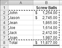
6. Select the cell(s) you want to include in the consolidation, including any text that identifies data (Figure 48). The text must be in cells adjacent to the data. The reference is entered into the Reference text box.
Figures 48, 49, & 50. Select the cell(s) you want to include in the consolidation.


7. Click Add.
8. Repeat steps 5, 6, and 7 for all cells you want to include in the consolidation. Figures 49 and 50 show the other two ranges included for the example. When you’re finished, the Consolidate dialog might look something like Figure 51.
Figure 51. The Consolidate dialog records all selections and enables you to specify where the data labels are.

9. Turn on the appropriate check box(es) in the Use labels in area to tell Excel where identifying labels for the data are.
10. Click OK.
Excel consolidates the information in the originally selected cell(s) (Figure 52).
Figure 52. The final consolidation accounts for all data.
Custom Views
Excel’s custom views feature lets you create multiple views of a workbook file. A view includes the window size and position, the active cell, the zoom percentage, hidden columns and rows, and print settings. Once you set up a view, you can choose it from a dialog to see it quickly.
• Including print settings in views makes it possible to create and save multiple custom reports for printing.
To add a custom view
1. Create the view you want to save. Figure 53 shows an example.
Figure 53. Create a view you’d like to save.

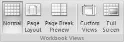
2. Click View > Workbook Views > Custom Views (Figure 54).
Figure 54. The Workbook Views group on the Ribbon’s View tab.
3. In the Custom Views dialog (Figure 55), click the Add button.
Figure 55. The Custom Views dialog before any views have been added.

4. In the Add View dialog (Figure 56), enter a name for the view in the Name text box.
Figure 56. Use the Add View dialog to name and set options for a view.
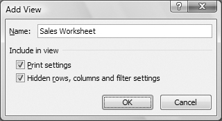
5. Turn on the appropriate Include in view check boxes:
• Print settings includes current Page Setup and other printing options in the view.
• Hidden rows, columns and filter settings includes current settings for hidden columns and rows, as well as filter selections.
6. Click OK.
To switch to a view
1. Switch to the sheet containing the view you want to see.
2. Click View > Workbook Views > Custom Views (Figure 54).
3. In the Custom Views dialog (Figure 57), select the view you want to see from the Views scrolling list.
Figure 57. To see or delete a view, select the name of the view in the Custom Views dialog, then click Show or Delete.

4. Click Show.
Excel changes the window so it looks just like it did when you created the view.
To delete a view
1. Switch to the sheet containing the view you want to delete.
2. Click View > Workbook Views > Custom Views (Figure 54).
3. In the Custom Views dialog (Figure 57), select the view you want to delete from the Views scrolling list.
4. Click Delete.
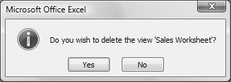
5. In the confirmation dialog that appears (Figure 58), click Yes.
Figure 58. When you click the Delete button to delete a view, Excel asks you to confirm that you really do want to delete it.
6. Follow steps 3 through 5 to delete other views if desired.
7. Click Close to dismiss the Custom Views dialog without changing the view.
• Deleting a view does not delete the information contained in the view. It merely removes the reference to the information from the Views list in the Custom Views dialog (Figure 57).
Macros
A macro is a series of commands that Excel can perform automatically. You can create simple macros to automate repetitive tasks, like entering data or formatting cells.
Although macros are created with Excel’s built-in Visual Basic programming language, you don’t need to be a programmer to create them. Excel’s Macro Recorder will record your keystrokes, menu choices, and dialog settings as you make them and will write the programming code for you. This makes macros useful for all Excel users, even beginners.
• The macro feature makes it possible to create highly customized workbook files, complete with special dialogs, menus, and commands. A discussion of these capabilities, however, is far beyond the scope of this book.
To record a macro
1. Choose View > Macros > Macros > Record Macro (Figure 59) to display the Record Macro dialog (Figure 60).
Figure 59. The Macros menu in the Macros group offers commands for working with—you guessed it—macros.
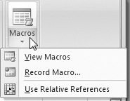
Figure 60. Enter a name and set options for a new macro in the Record Macro dialog.

2. Enter a name for the macro in the Macro name text box.
3. If desired, enter a keystroke to use as a shortcut key in the Ctrl+ text box.
4. If desired, edit the description automatically entered in the Description text box.
5. Click OK.
6. Perform all the steps you want to include in your macro. Excel records them all—even the mistakes—so be careful!
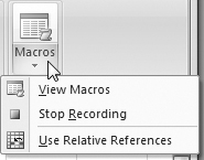
7. When you’re finished recording macro steps, choose View > Macros > Macros > Stop Recording (Figure 61).
Figure 61. When you’re finished recording macro steps, choose the Stop Recording command.
To run a macro
Press the keystroke you specified as a shortcut key for the macro when you created it.
Or
1. Choose View > Macros > Macros > View Macros (Figure 59).
2. In the scrolling list of the Macro dialog (Figure 62), select the macro you want to run.
Figure 62. The Macro dialog enables you to run, edit, and delete macros.
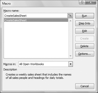
3. Click Run.
Excel performs each macro step, just the way you recorded it.
• Save your workbook before running a macro for the first time. You may be surprised by the results and need to revert the file to the way it was before you ran the macro. Excel’s Undo command cannot undo the steps of a macro, so reverting to the last saved version of the file is the only way to reverse macro steps.
• Excel stores each macro as a module within the workbook. View and edit a macro by selecting it in the Macro dialog and clicking the Edit button. Figure 63 shows an example. I don’t recommend editing macro code unless you have at least a general understanding of Visual Basic!
Figure 63. Here’s the code for a macro that adds formatted column and row headings to a blank worksheet.

• More advanced uses of macros include the creation of custom functions and applications that work within Excel.