
2. Worksheet Basics
How Worksheets Work
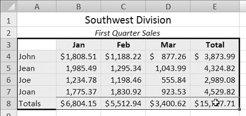
Microsoft Excel is most commonly used to create worksheets. A worksheet is a collection of information laid out in columns and rows. As illustrated in Figure 1, each worksheet cell can contain one of two kinds of input:
• A value is a piece of information that does not change. Values can be text, numbers, dates, or times. A cell containing a value usually displays the value.
• A formula is a collection of values, cell references, operators, and predefined functions that, when evaluated by Excel, produces a result. A cell containing a formula displays the results of the formula.
Figure 1. This very simple worksheet illustrates how a spreadsheet program like Excel works with values and formulas.

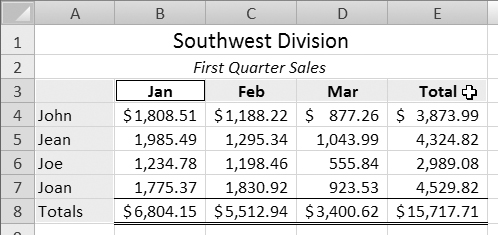
Although any information can be presented in a worksheet, spreadsheet programs like Excel are usually used to organize and calculate numerical or financial information. Why? Well, when properly prepared, a worksheet acts like a super calculator. You enter values and formulas and it calculates and displays the results. If you change one of the values, Excel automatically recalculates the results (Figure 2).
Figure 2. When the value for Sales changes from $1,000 to $1,150, the Profit result changes automatically.

How does this work? By using cell references rather than actual numbers in formulas, Excel knows that it should use the contents of those cells in its calculations. Thus, changing one or more values affects the results of calculations that include references to the changed cells. As you can imagine, this makes worksheets powerful business planning and analysis tools!
Starting Excel
To use Excel, you must start the Excel program. This loads Excel into RAM (random access memory), so your computer can work with it.
To run Excel from the Taskbar
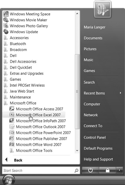
Click Start > All Programs > Microsoft Office > Microsoft Office Excel 2007 (Figure 3).
Figure 3. You can start Excel from the Start button on the Taskbar.
The Excel splash screen appears briefly, then an empty document window named Book1 appears (Figure 4).
Figure 4. When you start Excel from the Windows Taskbar, it displays an empty document window.

To run Excel by opening an Excel document
1. In Windows, locate the icon for the document that you want to open.
2. Double-click the icon.
The Excel splash screen appears briefly, then a document window containing the document that you opened appears.
• In Excel 2007, a document icon displays a preview of the worksheet or chart on the first sheet. Documents created with previous versions of Excel display standard Excel document icons (Figure 5).
Figure 5. A document created with a previous version of Excel has an icon like this one.

Exiting Excel
When you’re finished using Excel, you should use the Exit command to close the program. This completely clears Excel out of RAM, freeing up RAM for other programs.
To exit Excel
Choose Office button > Exit Excel (Figure 6). Here’s what happens:
• If any documents are open, they close.
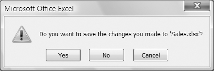
• If an open document contains unsaved changes, a dialog appears (Figure 7) so you can save the changes. I explain how to save documents in Chapter 4.
• The Excel program closes.
Figure 6. Excel’s Office button menu.

Figure 7. A dialog like this appears if a document with unsaved changes is open when you exit Excel.
• As you’ve probably guessed, Excel automatically exits when you restart or shut down your computer.
• Another way to Exit Excel is to click the Close button in the upper-right corner of Excel’s application window.
Creating a New Workbook
The documents you create and save using Excel are workbook files. A workbook is an Excel document.
In Excel, all workbooks are based on templates. A template is a file with built-in settings that control appearance and functionality. Some templates can include predefined contents such as values, formulas, formatting, and macros. Even a blank workbook file is based on a template—in this case, the Blank Workbook template.
Excel’s New Workbook dialog (Figure 8) offers several ways to create a workbook file:
• Blank and recent (Figure 8) makes it possible to create a workbook file based on the Blank Workbook template or any other recently used template.
• Installed Templates (Figure 9) lets you create a workbook file based on templates installed with Excel.
• My templates lets you create a workbook file based on templates you may have created or saved while working with Excel. You can also use this option to create a workbook based on a template created by someone else and accessible from your computer—such as a template designed by a co-worker for a specific company task.
• New from existing (Figure 14) enables you to create a workbook file based on an existing workbook. This makes it possible to duplicate a workbook without accidentally overwriting it with new information.
• Microsoft Office Online (Figure 11) lets you go online to the Microsoft Web site to choose a template from a wide variety of categories.
Figure 8. Creating a Blank Workbook with the New Workbook dialog.

Figure 9. The New Workbook dialog enables you to select from several installed templates.

• Basing a workbook on a template or existing workbook can save a lot of time if you need to create a standard document—such as a monthly report or invoice—repeatedly. Creating templates is covered in Chapter 4.
• Throughout this book, I often use the term document to refer to an Excel workbook file. For the purpose of this book, these terms are interchangeable.
• You can find more information about Excel workbook files in Chapter 4.
To create a blank workbook
1. Choose Office button > New to display the New Workbook dialog (Figure 8).
2. In the left panel, select Blank and recent.
3. In the center panel, select Blank Workbook.
4. Click Create.
A blank workbook window appears (Figure 4).
To create a workbook based on an installed template
1. Choose Office button > New to display the New Workbook dialog (Figure 8).
2. In the left panel, select Installed Templates.
3. In the Center Panel, select the icon for one of the installed templates. A preview of that template appears in the right panel (Figure 9).
4. Click Create.
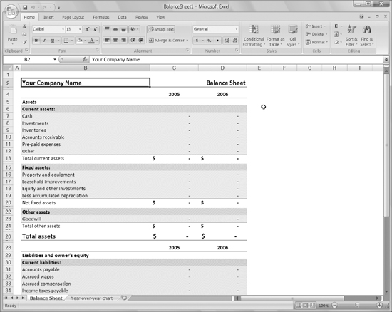
A workbook with the name of the template followed by a number appears (Figure 10). Make changes to the workbook as desired.
Figure 10. Here’s an example of a workbook based on one of the installed templates.
To create a workbook based on an online template
1. Choose Office button > New to display the New Workbook dialog (Figure 8).
2. In the left panel, select one of the categories under Microsoft Office Online.
3. If a list of links appears in the center panel, click the link for the subcategory you want.
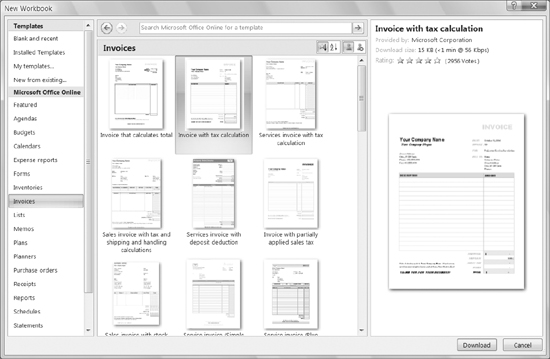
4. In the center panel, select the icon for one of the templates. A preview of that template appears in the right panel (Figure 11).
Figure 11. You can also access templates from Microsoft Office Online.
5. Click Download.
A workbook with the name of the template followed by a number appears (Figure 12). Make changes to the workbook as desired.
Figure 12. Here’s an example of a workbook created from an online template.

• You must have an Internet connection to create a workbook based on a template on the Microsoft Office Online Web site.
• After step 4, a dialog may appear, informing you that templates are only available to customers running Genuine Microsoft Office (Figure 13). To never see this dialog again, turn on the Do not show this message again check box and click Continue.
Figure 13. Excel may display this dialog to let you know that you must have a “genuine” copy of Office to download templates.

To create a workbook based on an existing workbook
1. Choose Office button > New to display the New Workbook dialog (Figure 8).
2. In the left panel, select New from existing.
3. The New from Existing Workbook dialog appears (Figure 14). Use it to locate and select the workbook you want to base a new workbook on.
Figure 14. The New from Existing Workbook dialog enables you to choose an existing workbook on which to base a new one.

4. Click Create New.
A workbook with the name of the existing document followed by a number appears (Figure 15). Make changes to the workbook as desired.
Figure 15. The existing workbook appears with a new name so you can change it and save it as a new file.

• The New from Existing Workbook dialog (Figure 14) is very similar to the Open dialog, which I cover in Chapter 4.
• This is the best way to create a new workbook from an existing workbook. If you simply open an existing workbook and make changes to it, you might accidentally overwrite the original workbook when you save the new one.
Activating & Selecting Cells
Worksheet information is entered into cells. A cell is the intersection of a column and a row. Each little “box” in the worksheet window is a cell.
Each cell has a unique address or reference. The reference uses the letter(s) of the column and the number of the row. Thus, cell B6 would be at the intersection of column B and row 6. The reference for the active cell appears in the name box at the left end of the formula bar (Figure 16).
Figure 16. The reference for an active cell appears in the formula bar.

To enter information in a cell, you must make that cell active. When a cell is active, anything you type is entered into it.
To use Excel commands on a cell or its contents, you must select the cell. The active cell is also a selected cell. If desired, however, you can select multiple cells or a range of cells. This enables you to use commands on all selected cells at once. A range (Figure 17) is a rectangular selection of cells defined by the top-left and bottom-right cell references.
Figure 17. In this illustration, the range A3:B8 is selected, and cell A3 is the active cell.

• Although the active cell is always part of a selection of multiple cells, it is never highlighted like the rest of the selection (Figure 17).
• Although you can select multiple cells, only one cell—the one referenced in the name box (Figure 17)—is active.
• The column and row headings for selected cells appear colored (Figures 16 and 17).
• Using the scroll bars does not change the active or selected cell(s). It merely changes your view of the worksheet’s contents.
To activate a cell
Use the mouse pointer to click in the cell.
Or
Press the appropriate keystroke (Table 1) to move the cell pointer.
Table 1. Keys for Moving the Cell Pointer

To select a range of cells with the mouse
1. Position the mouse pointer in the first cell you want to select (Figure 18).
Figure 18. To select cells, begin in one corner of the range...

2. Hold the mouse button down and drag to highlight all the cells in the selection (Figure 19).
Figure 19. ... hold the mouse button down, and drag to the opposite corner of the range.
Or
1. Click in the first cell of the range you want to select.
2. Hold down ![]() and click in the last cell of the range. Everything between the first and second clicks is selected. (This technique is known as shift-click.)
and click in the last cell of the range. Everything between the first and second clicks is selected. (This technique is known as shift-click.)
To go to a cell or range of cells
1. Choose Home > Editing > Find & Select > Go To (Figure 20) or press ![]() to display the Go To dialog (Figure 21).
to display the Go To dialog (Figure 21).
Figure 20. Choose Go To from the Find & Select menu.

Figure 21. The Go To dialog lets you move to any cell quickly.

2. Enter the reference for the cell you want to activate or the range that you want to select in the Reference text box.
3. Click OK. If you entered a single cell reference, the cell is activated. If you entered a range reference, the range is selected.
• To specify a reference for a range, enter the addresses of the first and last cells of the range, separated with a colon (:). For example, Figure 17 shows A3:B8 selected and Figure 19 shows A3:E8 selected.
To select an entire column
1. Position the mouse pointer on the heading for the column you want to select. The mouse pointer turns into an arrow pointing down (Figure 22).
Figure 22. Click a column heading to select the column.

2. Click once. The column is selected.
To select an entire row
1. Position the mouse pointer on the heading for the row you want to select. The mouse pointer turns into an arrow pointing to the right (Figure 23).
Figure 23. Click a row heading to select the row.

2. Click once. The row is selected.
To select multiple columns or rows
1. Position the mouse pointer on the first column or row heading.
2. Press the mouse button down, and drag along the headings until all the desired columns or rows are selected.
• When selecting multiple columns or rows, be careful to position the mouse pointer on the heading and not between two headings! If you drag the border of two columns, you will change a column’s width rather than make a selection.
To select the entire worksheet
1. Position the mouse pointer on the Select All button in the upper-left corner of the worksheet window. The mouse pointer appears as a hollow plus sign (Figure 24).
Figure 24. Click the Select All button to select all cells in the worksheet.

2. Click once.
Or
Press ![]() .
.
The worksheet is selected.
To select multiple ranges
1. Use any selection technique to select the first cell or range of cells (Figure 25).
Figure 25. To select two ranges of cells, start by selecting the first range, ...

2. Hold down ![]() and drag to select the second cell or range of cells (Figure 26).
and drag to select the second cell or range of cells (Figure 26).
Figure 26. ... then hold down ![]() and select the second range.
and select the second range.
3. Repeat step 2 until all desired ranges are selected.
• Selecting multiple ranges can be tricky. It takes practice. Don’t be frustrated if you can’t do it on the first few tries!
• To add ranges that are not visible in the worksheet window, be sure to use the scroll bars to view them. Using the keyboard to move to other cells while selecting multiple ranges will remove the selections you’ve made so far or add undesired selections.
• Do not click in the worksheet window or use the movement keys while multiple ranges are selected unless you are finished working with them. Doing so will deselect all the cells.
To deselect cells
Click anywhere in the worksheet.
Or
Press any of the keys in Table 1.
Entering Values & Formulas
To enter a value or formula into a cell, begin by making the cell active. As you type or click to enter information, the information appears in both the cell and in the formula bar just above the window’s title bar. You complete the entry by pressing ![]() or clicking the Enter button on the formula bar.
or clicking the Enter button on the formula bar.
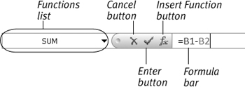
While you are entering information into a cell, the formula bar is active. You can tell that it’s active because the name box on the left end of the formula bar turns into a Functions list and two additional buttons appear between it and the cell contents area (Figure 27).
Figure 27. The individual components of the formula bar.
There are two important things to remember when the formula bar is active:
• Anything you type or click on may be included in the active cell.
• Some Excel options and menu commands are unavailable.
You deactivate the formula bar by accepting or cancelling the current entry.
• Pressing ![]() to complete a formula entry accepts the entry and moves the cell pointer one cell down. Clicking the Enter button accepts the entry without moving the cell pointer.
to complete a formula entry accepts the entry and moves the cell pointer one cell down. Clicking the Enter button accepts the entry without moving the cell pointer.
• To cancel an entry before it has been completed, press ![]() or click the Cancel button on the formula bar. This restores the cell to the way it was before you began.
or click the Cancel button on the formula bar. This restores the cell to the way it was before you began.
• If you include formatting notation such as dollar signs, commas, and percent symbols when you enter numbers, Excel may apply formatting styles. Formatting the contents of cells is discussed in Chapter 6.
Values
As discussed at the beginning of this chapter, a value is any text, number, date, or time you enter into a cell. Values are constant—they don’t change unless you change them.
To enter a value
1. Activate the cell in which you want to enter the value.
2. Type in the value. As you type, the information appears in two places: the active cell and the formula bar, which becomes active (Figure 28).
Figure 28. As data is entered into a cell, it appears in the cell and in the formula bar.

3. To complete and accept the entry (Figure 29), press ![]() , or click the Enter button on the formula bar.
, or click the Enter button on the formula bar.
Figure 29. A completed entry. The insertion point is gone.

• Although you can often use the arrow keys or other movement keys in Table 1 to complete an entry by moving to another cell, it’s a bad habit because it won’t always work.
• Pressing ![]() to complete an entry automatically advances the cell pointer to the next cell.
to complete an entry automatically advances the cell pointer to the next cell.
• By default, Excel aligns text against the left side of the cell and aligns numbers against the right side of the cell. I explain how to change alignment in Chapter 6.
• Don’t worry if the data you put into a cell doesn’t seem to fit. You can always change the column width or use the AutoFit Text feature to make it fit. I explain how in Chapter 6.
Formula Basics
Excel makes calculations based on formulas you enter into cells. When you complete the entry of a formula, Excel displays the results of the formula rather than the formula.
Here are some important things to keep in mind when writing formulas:
• If a formula uses cell references to refer to other cells and the contents of one or more of those cells changes, the result of the formula changes, too.
• All formulas begin with an equal (=) sign. This is how Excel knows that a cell entry is a formula and not a value.
• Formulas can contain any combination of values, references, operators (Table 2), and functions. I tell you about using operators in formulas in this chapter and about using functions in Chapter 5.
Table 2. Basic Mathematical Operators Understood by Excel

• Formulas are not case sensitive. This means that =A1+B10 is the same as =a1+b10. Excel automatically converts characters in cell references and functions to uppercase.
When calculating the results of expressions with a variety of operators, Excel makes calculations in the following order:
1. Negation
2. Expressions in parentheses
3. Percentages
4. Exponentials
5. Multiplication or division
6. Addition or subtraction
Table 3 shows some examples of formulas and their results to illustrate this. As you can see, the inclusion of parentheses can really make a difference when you write a formula!
Table 3. How Excel Evaluates Expressions

• Do not use the arrow keys or other movement keys to complete an entry by moving to another cell. Doing so may add cells to the formula!
• Whenever possible, use references rather than values in formulas. This way, you won’t have to rewrite formulas when values change. Figures 30 and 31 illustrate this.
Figure 30. If any of the values change, the formulas will need to be rewritten!

Figure 31. But if the formulas reference cells containing the values, when the values change, the formulas will not need to be rewritten to show correct results.

• A reference can be a cell reference, a range reference, or a cell or range name. I tell you about name references in Chapter 13.
• To add a range of cells to a formula, type the first cell in the range followed by a colon (:) and then the last cell in the range. For example, B1:B10 references the cells from B1 straight down through B10.
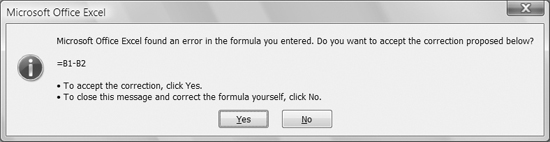
• If you make a syntax error in a formula, Excel tells you (Figures 32, 33, and 34). If the error is one of the common errors programmed into Excel’s Formula AutoCorrect feature, Excel offers to correct the formula for you (Figure 34). Otherwise, you will have to troubleshoot the formula and correct it yourself.
Figure 32. Excel tells you when a formula has an error and provides information on where you can get help.

Figure 33. This dialog appears when a formula contains a circular reference—a reference to its own cell.
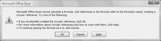
Figure 34. If the error is one of the common formula errors Excel knows about, Excel offers to fix it for you.
• I explain how to edit formulas in Chapter 3 and how to include functions in formulas in Chapter 5.
To enter a formula by typing
1. Activate the cell in which you want to enter the formula.
2. Type in the formula. As you type, the formula appears in two places: the active cell and the formula bar (Figure 35).
Figure 35. To enter a formula, type it into a cell.

3. To complete the entry (Figure 36), press ![]() or click the Enter button on the formula bar.
or click the Enter button on the formula bar.
Figure 36. A completed formula entry.

• As you type cell references, Excel may attempt to suggest functions you might be trying to type. These functions will appear in a drop-down list, as shown in Figure 37. You can ignore this list; it will disappear as you type. I tell you how to use functions in Chapter 5.
Figure 37. If you type a cell reference in a formula, Excel assumes you’re trying to type in a function and suggests a few.

To enter a formula by clicking
1. Activate the cell in which you want to enter the formula.
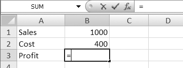
2. Type an equal (=) sign to begin the formula (Figure 38).
Figure 38. To enter the formula =B1–B2, type = to begin the formula, ...
3. To enter a cell reference, click on the cell you want to reference (Figures 39 and 41).
or
To enter a constant value or operator, type it in (Figure 40).
Figure 39. ... click cell B1 to add its reference to the formula, ...

Figure 40. ... type – to tell Excel to subtract, ...
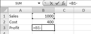
Figure 41. ... click cell B2 to add its reference to the formula, ...

4. Repeat step 3 until the entire formula appears in the formula bar.
5. To complete the entry (Figure 42), press ![]() or click the Enter button on the formula bar.
or click the Enter button on the formula bar.
Figure 42. ... and finally, click the Enter button to complete the formula.

• If you click a cell reference without typing an operator, Excel assumes you want to add that reference to the formula.
• Be careful where you click when writing a formula! Each click adds a reference to the formula. If you add an incorrect reference, press ![]() until it has been deleted or click the Cancel button on the formula bar to start the entry from scratch. I explain how to edit a cell’s contents in Chapter 3.
until it has been deleted or click the Cancel button on the formula bar to start the entry from scratch. I explain how to edit a cell’s contents in Chapter 3.
• You can add a range of cells to a formula by dragging over the cells.
Error Checking Smart Tags
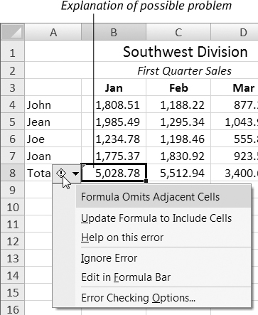
Excel’s Error Checking Smart Tag feature alerts you to possible errors in cells. For example, suppose you write a formula that sums all the numbers in a column, but you leave out the last cell reference for the last cell in the column. Excel assumes this is an error and marks the cell with a small green triangle in the upper-left corner of the cell (Figure 43). When you select the cell, a Smart Tag icon appears beside it (Figure 44). Clicking the Smart Tag displays a menu of options for correcting, learning more about, or ignoring the possible error (Figure 45).
Figure 43. A tiny green error marker appears in the corner of a cell that contains a possible error.
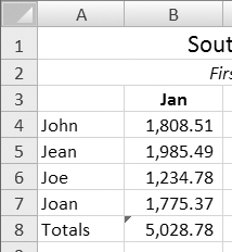
Figure 44. When you activate a cell with a possible error, the Error Checking Smart Tag icon appears.

Figure 45. Choose an option from the Smart Tag menu to resolve the possible error.
To correct an error with a Smart Tag
1. Click the Smart Tag icon that appears beside a cell with a possible error (Figure 44). A menu of options appears (Figure 45).
2. Choose the option immediately below the description of the error.
To ignore an error & remove its Smart Tag
1. Click the Smart Tag icon that appears beside a cell with a possible error (Figure 44). A menu of options appears (Figure 45).
2. Choose Ignore Error. The Smart Tag and green triangle disappear.