
11. Working with Others
Collaboration Features
In office environments, a document is often the product of multiple people. In the old days, a draft worksheet or financial report would be printed and circulated among reviewers. Along the way, it would be marked up with colored ink and covered with sticky notes full of comments. Some poor soul would have to make sense of all the markups and notes to create a clean document. The process was time consuming and was sometimes repeated through several drafts to fine-tune the document for publication.
Microsoft Excel, which is widely used in office environments, includes many features that make the collaboration process easier:
• Properties stores information about the document’s creator and contents.
• Comments enables reviewers to enter notes about the document. The notes don’t print—unless you want them to.
• Change Tracking enables reviewers to edit the document while keeping the original document intact. Changes can be accepted or rejected to finalize the document.
• Document Protection limits how a document can be changed.
• Workbook sharing enables multiple users to access a workbook file simultaneously via network.
• Save options protect documents from being opened or modified.
Document Properties
The Document Properties pane (Figure 1) enables you to store information about a document. This information, which is saved with the document, can be viewed by anyone who opens the document.
Figure 1. The Document Properties pane, which appears above the document window, offers text boxes for entering information about the document.

• Information in the Document Properties pane is also used by Microsoft’s search feature. A discussion of this feature is beyond the scope of this book, but you can see it in action by clicking Start and entering search criteria in the Start Search box.
To view, enter, or edit Document Properties information
1. Open the document for which you want to view or edit properties.
2. Choose Microsoft Office > Prepare > Properties (Figure 2). The Document Properties pane appears above the document (Figure 1).
Figure 2. The Prepare submenu on the Microsoft Office menu.

3. Enter or edit information in each field as desired:
• Author is the person who created the document. This field may already be filled in based on information stored in Excel.
• Title is the title of the document. This does not have to be the same as the file name.
• Subject is the subject of the document.
• Keywords are important words related to the document.
• Category is a category name assigned to the document. It can be anything you like.
• Status is the document’s status.
• Comments are notes about the document.
4. When you are finished viewing or editing Document Properties pane contents, click the pane’s close button. Your changes are automatically saved.
• It is not necessary to enter information in every text box.
• Excel’s Properties dialog (Figure 3) offers additional information about a document. To open it, choose Advanced Properties from the Document Properties pop-up menu in the upper-left corner of the Document Properties pane.
Figure 3. The General tab of the Properties dialog for a workbook. Other tabs show additional information.

Comments
Comments are annotations that you and other document reviewers can add to a document. These notes can be viewed onscreen but don’t print unless you want them to.
To insert a comment
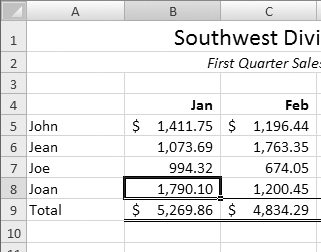
1. Select the cell for which you want to insert a comment (Figure 4).
Figure 4. Start by selecting the cell you want to enter a comment for.
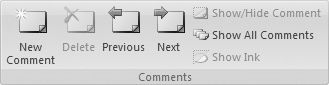
2. Choose Review > Comments > New Comment (Figure 5).
Figure 5. The Review tab’s Comments group.
Two things happen: a comment marker (a tiny red triangle) appears in the upper-right corner of the cell and a box with your name and a blinking insertion point appears (Figure 6).
Figure 6. Excel prepares to accept your comment.

3. Type your comment into the box. It can be as long or as short as you like (Figure 7).
Figure 7. Enter your comment in the box.

4. When you are finished, click anywhere else in the worksheet window. Your comment is saved and the box disappears.
To view comments
Position the mouse pointer over a cell with a comment marker. A box appears containing the name of the person who wrote the comment and the comment itself (Figure 8).
Figure 8. When you position the mouse pointer over a cell with a comment marker, the comment appears.

Or
Click Review > Comments > Show All Comments (Figure 5). All comments for visible cells appear in yellow boxes (Figure 9).
Figure 9. When you click the Show All Comments button, all comments for visible cells appear.

Or
To show or hide a specific comment select the cell containing the comment and click Review > Comments > Show/Hide Comment (Figure 5).
• If all comments are displayed, you can hide them by clicking Review > Comments > Show All Comments.
To edit a comment
1. Select the cell containing the comment you want to edit.
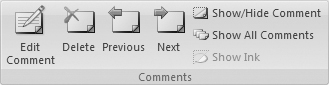
2. Click Review > Comments > Edit Comment (Figure 10).
Figure 10. The Comments group with a cell containing a comment selected.
3. Edit the contents of the comment box (Figure 7).
4. When you are finished, click anywhere else in the worksheet window. Your comment is saved and the box disappears.
To delete a comment
1. Select the cell containing the comment you want to remove.
2. Choose Review > Comments > Delete (Figure 10). The comment marker and comment are removed.
To print comments
1. Follow the instructions in Chapter 9 to prepare the sheet for printing and open the Page Setup dialog.
2. Choose an option from the Comments drop-down list in the Sheet tab (Figure 11).
Figure 11. Choose an option from the Comments drop-down list.

3. Click Print.
4. In the Print dialog that appears, click OK to print the sheet and its comments.
Change Tracking
Excel’s revision tracking feature enables multiple reviewers to edit a document without actually changing it. Instead, each reviewer’s markups are displayed in the document window. At the conclusion of the reviewing process, someone with final say over document content reviews all of the edits and either accepts or rejects each of them. The end result is a final document that incorporates the accepted changes.
To turn change tracking on or off
1. Choose Review > Changes > Track Changes > Highlight Changes (Figure 12).
Figure 12. Choose Highlight Changes from the Track Changes menu to enable the change tracking feature.

2. In the Highlight Changes dialog that appears (Figure 13), toggle check boxes to set up the revision tracking feature:
• Track changes while editing enables the revision tracking feature. Turn on this check box to track changes. Turn off this check box to disable the revision tracking feature.
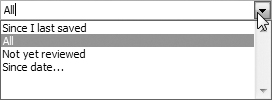
• When enables you to choose which changes should be tracked based on when the changes were made. If you turn on this check box, choose an option from the drop-down list (Figure 14).
• Who enables you to specify which changes should be tracked based on who made them. If you turn on this check box, choose an option from the drop-down list (Figure 15).
• Where enables you to specify which changes should be tracked based on which cells the changes were made in. If you turn on this check box, enter a range of cells in the text box beside it.
• Highlight changes on screen displays revision marks in the document window.
• List changes on a new sheet records changes in a separate History worksheet. This option is only available after you have saved the workbook file as a shared workbook.
Figure 13. The Highlight Changes dialog lets you enable and configure the revision tracking feature.

Figures 14 & 15. Use these two drop-down lists to specify which changes to track based on when they were made (top) or who made them (bottom).

3. Click OK.
4. If prompted, save the workbook file.
• Turning on revision tracking also shares the workbook file. I tell you more about workbook sharing later in this chapter.
To track changes
1. Turn on revision tracking as instructed on the previous page.
2. Make changes to the document.
The cells you changed get a colored border around them and a color-coordinated triangle appears in the upper-left corner (Figure 16).
Figure 16. When you edit the document, the cells you change are marked.

• If the document is edited by more than one person, each person’s revision marks appear in a different color. This makes it easy to distinguish one editor’s changes from another’s.
To view revision information
Point to a revision mark. A box with information about the change appears (Figure 17).
Figure 17. Point to a revision mark to display information about it.

To accept or reject revisions
1. Choose Review > Changes > Track Changes > Accept/Reject Changes (Figure 18).
Figure 18. Choose Accept/Reject Changes from the Track Changes menu.

2. If prompted, save the workbook file.
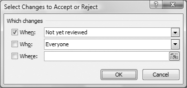
3. The Select Changes to Accept or Reject dialog appears (Figure 19). Set options to select the changes to review. The options work like those in the Highlight Changes dialog (Figure 13).
Figure 19. The Select Changes to Accept or Reject dialog.
4. Click OK.
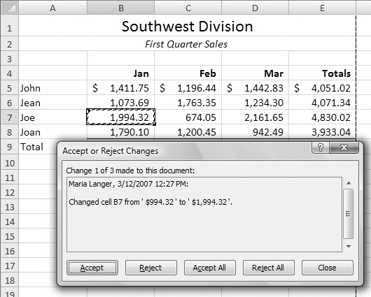
5. Excel selects the first change and displays the Accept or Reject Changes dialog (Figure 20).
• To accept the currently selected change, click the Accept button. Excel selects the next change.
• To reject the currently selected change, click the Reject button. The cell reverts to its original contents and Excel selects the next change.
• To accept all changes, click the Accept All button. Skip the remaining step.
• To reject all changes, click the Reject All button. All changed cells in the selection revert to their original contents. Skip the remaining step.
Figure 20. Excel selects the changed cell and displays information about the change in the Accept or Reject Changes dialog.
6. Repeat step 5 for each change Excel selects.
When Excel has reached the end of the document, the Accept or Reject Changes dialog disappears.
• The Undo command will not work after you click the Accept All or Reject All button in step 5. Use these two buttons with care!
To remove revision marks
1. Choose Review > Changes > Track Changes > Highlight Changes (Figure 12).
2. In the Highlight Changes dialog (Figure 13), turn off the Track changes while editing check box and click OK.
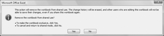
3. A dialog like the one in Figure 21 may appear. You have two options:
• Yes turns off workbook sharing.
• No keeps the workbook sharing turned on.
Figure 21. This dialog may appear when you turn off the change tracking feature.
The revision marks disappear.
• Removing the revision marks also turns off the change tracking feature.
• I tell you more about workbook sharing later in this chapter.
Document Protection
Excel’s document protection features enable you to limit the types of changes others can make to a document. There are four types of protection:
• Protect Sheet protects against certain types of changes to worksheets and locked worksheet cells.
• Allow Users to Edit Ranges protects against changes to specific ranges of worksheet cells.
• Protect Workbook protects workbook structure and windows.
• Protect and Share Workbook enables you to share the workbook but only with change tracking enabled.
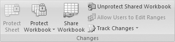
You set up all protection options using commands in the Review tab’s Changes group (Figure 22).
Figure 22. The Review tab’s Changes group.

• I explain how revision tracking works earlier in this chapter.
• I tell you more about sharing workbooks without enabling protection later in this chapter.
• In addition to document protection, you can password protect a document to prevent it from being opened or changed. I explain how later in this chapter.
• If you use the Information Rights Management service offered by Microsoft, you can set other protection options for your Excel workbook files. A discussion of this fee-based service is beyond the scope of this book.
To protect a sheet
1. Click Review > Changes > Protect Sheet (Figure 22).
2. In the Protect Sheet dialog that appears (Figure 23), turn on check boxes for the types of changes you want to allow.
Figure 23. Use the Protect Sheet dialog to set protection options for the active worksheet.

3. If desired, enter a password in the Password text box.
4. Click OK.
5. If you entered a password, the Confirm Password dialog appears (Figure 24). Enter the password again and click OK.
Figure 24. If you entered a password in the Protect Sheet dialog, you’ll have to enter it again to turn on protection.

• Entering a password in the Protect Sheet dialog (Figure 23) is optional. If you do not use a password, however, the document can be unprotected by anyone.
• If you enter a password in the Protect Sheet dialog (Figure 23), don’t forget it! If you can’t remember the password, you can’t unprotect the document!
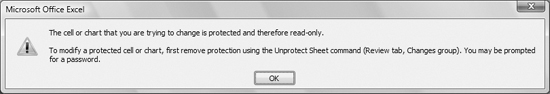
• If you try to change a protected item, Excel displays a dialog reminding you that the item is protected (Figure 25).
Figure 25. Excel tells you when you’re trying to edit a protected item.
To unprotect a sheet
1. Click Review > Changes > Unprotect Sheet (Figure 26).
Figure 26. When a sheet is protected, the Protect Sheet button turns into a Unprotect Sheet button.

2. If protection is enforced with a password, enter the password in the Unprotect Sheet dialog that appears and click OK.
To turn off protection for selected cells
1. If the sheet is already protected, unprotect it.
2. Select the cells you want to allow modification to.
3. Choose Home > Cells > Format > Format Cells (Figure 27) to display the Format Cells dialog and click the Protection tab (Figure 28).
Figure 27. The Cells group’s Format menu.

Figure 28. Turn off the Locked check box to allow modification to selected cells in a protected sheet.
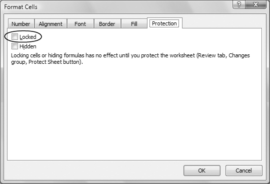
4. Turn off the Locked check box.
5. Click OK.
When you protect the sheet’s contents, the unlocked cells can be modified.
To allow users to edit ranges of a protected sheet
1. If the sheet is already protected, unprotect it.
2. Click Review > Changes > Allow Users to Edit Ranges (Figure 22). The Allow Users to Edit Ranges dialog appears (Figure 29).
Figure 29. The Allow Users to Edit Ranges dialog before any ranges have been defined.

3. To add an editable range of cells, click New to display the New Range dialog (Figure 30).
Figure 30. The New Range dialog with information for a range already entered.
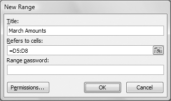
4. Enter information into each text box:
• Title is a name for the range.
• Refers to cells is the cell reference for the range.
• Range password is the password that allows you to edit the range of cells.
5. Click OK.
6. If you entered a password in step 4, the Confirm Password dialog appears (Figure 24). Enter the password again and click OK.
7. Repeat steps 2 through 6 for each range you want to add. The ranges appear in the Allow Users to Edit Ranges dialog (Figure 31).
Figure 31. Ranges you add appear in the Allow Users to Edit Ranges dialog.

8. Click OK.
9. Follow the instructions earlier in this section to protect the worksheet.
• In step 4, an easy way to enter the cell reference is to move the dialog aside and select the range in the worksheet window.
• Not entering a password in step 4 is the same as simply unlocking the cell. I explain how to turn off protection for selected cells earlier in this section.
• You can modify or delete the settings for a range by selecting the range name in the Allow Users to Edit Ranges dialog (Figure 31) and clicking either the Modify or the Delete button.
• If you turn on the Paste permissions information into a new workbook check box in the Allow Users to Edit Ranges dialog (Figure 31), Excel creates a worksheet with a summary of permissions settings (Figure 32).
Figure 32. Excel can record permission information in a worksheet.

• If you attempt to edit a cell that is part of a password-protected range in a protected worksheet, the Unlock Range dialog appears (Figure 33). Enter the appropriate password and click OK to edit the cell.
Figure 33. Enter the password assigned to the range to modify a cell within it.

• Excel’s permissions feature lets you further customize who can modify cell contents. Although this advanced feature is far beyond the scope of this book, you can experiment with it by clicking the Permissions button in the Allow Users to Edit Ranges (Figure 31) or New Range (Figure 30) dialogs.
To protect a workbook
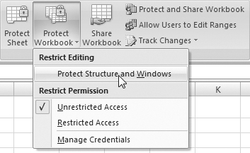
1. Choose Review > Changes > Protect Workbook > Protect Structure and Windows (Figure 34).
Figure 34. Choose Protect Structure and Windows.
2. In the Protect Structure and Windows dialog that appears (Figure 35), turn on check boxes for the type of protection you want:
• Structure prevents workbook sheets from being inserted, deleted, moved, hidden, unhidden, or renamed.
• Windows protects workbook windows from being moved, resized, hidden, unhidden, or closed.
Figure 35. Use the Protect Structure and Windows dialog to protect a workbook’s structure or windows.

3. If desired, enter a password in the Password text box.
4. Click OK.
5. If you entered a password in step 3, enter the password again in the Confirm Password dialog that appears (Figure 24) and click OK.
• With workbook protection options enabled, Excel disables any menu commands or shortcut keys that you would use to make unallowed changes.
To unprotect a workbook
1. Choose Review > Changes > Protect Workbook > Protect Structure and Windows (Figure 34).
2. If protection is enforced with a password, enter the password in the dialog that appears and click OK.
To protect a workbook for sharing & change tracking
1. Click Review > Changes > Protect and Share Workbook (Figure 22).
2. In the Protect Shared Workbook dialog that appears (Figure 36), turn on the Sharing with track changes check box.
Figure 36. Use the Protect Shared Workbook dialog to allow others to share the workbook, but only with change tracking enabled.
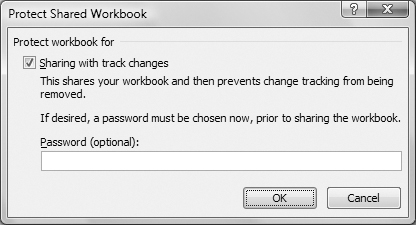
3. If desired, enter a password in the Password text box.
4. Click OK.
5. If you entered a password in step 3, enter the password again in the Confirm Password dialog that appears (Figure 24) and click OK.
6. When prompted to save the workbook, click OK. Excel turns on change tracking and workbook sharing.
• I tell you about workbook sharing later in this chapter and about change tracking earlier in this chapter.
To turn off workbook sharing & change tracking protection
1. Click Review > Changes > Unprotect Shared Workbook (Figure 37).
Figure 37. The Unprotect Shared Workbook command in the Changes group.
2. If protection is enforced with a password, enter the password in the dialog that appears and click OK.
Workbook Sharing
Excel’s workbook sharing feature enables multiple people to work on the same workbook at the same time. This feature is designed for work environments with networked computer systems.
To share a workbook
1. Click Review > Changes > Share Workbook (Figure 22).
2. In the Share Workbook dialog that appears, click the Editing tab to display its options (Figure 38).
Figure 38. Sharing a workbook is as easy as turning on a check box.

3. Turn on the check box beside Allow changes by more than one user at the same time.
4. Click OK.
5. A dialog prompts you to save the workbook. Click OK.
• You can identify a workbook that has sharing enabled by the word “Shared” in its title bar (Figure 39).
Figure 39. You can identify a shared workbook by the word “Shared” in its title bar.
![]()
To open a shared workbook
1. Choose Microsoft Office > Open (Figure 40).
Figure 40. The Microsoft Office menu.

2. Use the Open dialog that appears to open the network volume on which the workbook resides, then locate, select, and open the file.
To stop sharing a workbook
1. Click Review > Changes > Share Workbook (Figure 22).
2. In the Share Workbook dialog that appears, click the Editing tab to display its options (Figure 41).
Figure 41. The Share Workbook dialog lists all users who have the workbook file open.

3. To stop a specific user from sharing the workbook, select the user’s name from the user list and click the Remove User button. Then click OK in the warning dialog that appears.
or
To stop all users from sharing the workbook, turn off the check box beside Allow changes by more than one user at the same time.
4. Click OK.
5. A dialog may prompt you to save the workbook. Click OK.
• The Share Workbook dialog for a file lists all of the users who have the file open (Figure 41).
• If you remove a user from workbook sharing, when he tries to save the workbook, a dialog appears, telling him that he is no longer sharing the workbook and offering instructions on how to save his changes.
General Save Options & Password Protection
Excel’s general save options enable you to set up passwords to prevent a document from being opened or from being modified.
To set save options
1. Click Microsoft Office > Save As (Figure 40).
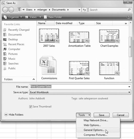
2. In the Save As dialog that appears, choose General Options from the Tools menu (Figure 42).
Figure 42. Choose General Options from the Tools menu in the Save As dialog.
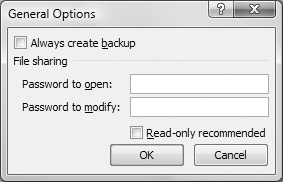
3. Set options in the General Options dialog (Figure 43) as desired:
• Always create backup tells Excel to save the previous version of the file as a backup when saving the current version. (The old file is named “Backup of filename.”)
• Password to open is the password that must be entered in order to open the file.
• Password to modify is the password that must be entered in order to save changes to the file.
• Read-only recommended tells Excel to recommend that the file be opened as a read-only file when the user tries to open it.
Figure 43. Use the General Options dialog to set all kinds of options for protecting a file.
4. Click OK.
5. If you entered a password in step 3, a dialog appears, asking you to confirm it (Figure 24). Re-enter the password and click OK. (If you entered two passwords, this dialog appears twice.)
To open a file that has general save options set
• If the file requires a password to open it, a dialog like the one in Figure 44 appears. Enter the password and click OK.
Figure 44. Use a dialog like this to enter a password to open a file.

• If the file requires a password for modification, a dialog like the one in Figure 45 appears. You have two choices:
• Enter the password and click OK.
• Click Read Only to open the file as a read-only file.
Figure 45. Use a dialog like this to enter a password to open a file for modification.

• If the file was set up so read-only access is recommended, a dialog like the one in Figure 46 appears, asking if you want to open the file as a read-only file. You have three choices:
• Click Cancel to not open the file at all.
• Click No to open the file as a regular file.
• Click Yes to open the file as a read-only file.
Figure 46. If read-only access is recommended for a file, Excel displays a dialog like this one when you open it.

• If a file is opened for read-only access, you cannot save changes to the file—a dialog like the one in Figure 47 appears if you try.
Figure 47. Excel displays a dialog like this if you try to save a file that is opened for read-only access.

• You can identify a file opened as a read-only file by the words “Read-Only” in the document window’s title bar (Figure 48).
Figure 48. Not sure if a document is open as a read-only file? Just look in the title bar.
![]()