6. Formatting Cells
Formatting Basics
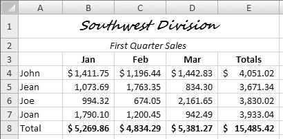
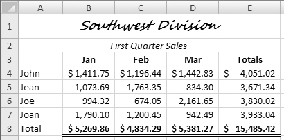
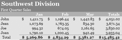
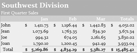
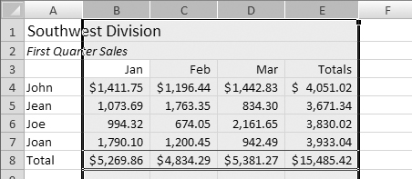
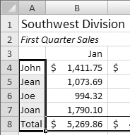
To paraphrase an old Excel mentor of mine, formatting a worksheet is like putting on its makeup. The worksheet’s contents may be perfectly correct, but by applying formatting, you can make a better impression on the people who see it (Figures 1 and 2).
Figure 1. While content should be more important than appearance, you can bet that this worksheet won’t get as much attention ...
Excel offers a wide range of formatting options you can use to beautify your worksheets:
• Number formatting lets you change the appearance of numbers, dates, and times.
• Alignment lets you change the way cell contents are aligned within the cell.
• Font formatting lets you change the appearance of text and number characters.
• Borders let you add lines around cells.
• Fill lets you add color, shading, and patterns to cells.
• Column and row formatting let you change column width and row height.
You can apply formatting to cells using a variety of techniques: with Formatting toolbar buttons, shortcut keys, menu commands, or the Conditional Formatting or AutoFormat features.
• Excel may automatically apply formatting to cells, depending on what you enter. For example, if you use a date function, Excel formats the results of the function as a date. You can change Excel’s formatting at any time to best meet your needs.
• Most formatting is applied to cells, not cell contents. If you use the Clear Contents command to clear a cell, the formatting remains and will be applied to whatever data is next entered into it.
Number Formatting
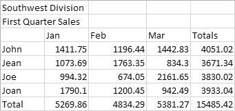
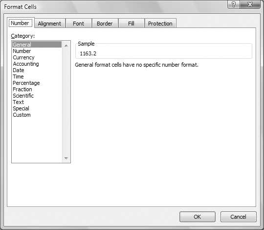
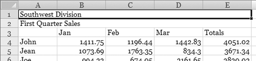
By default, Excel applies the General number format to worksheet cells. This format displays numbers just as they’re entered (Figure 3).
Figure 3. General formatting displays the numbers just as they’re typed in and uses scientific notation when they’re very big.

Excel offers a wide variety of predefined number formatting options for different purposes:
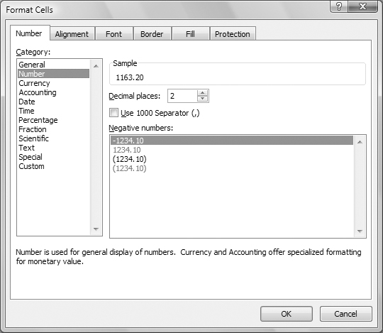
• Number formats are used for general number display.
• Currency formats are used for monetary values.
• Accounting formats are used to line up columns of monetary values.
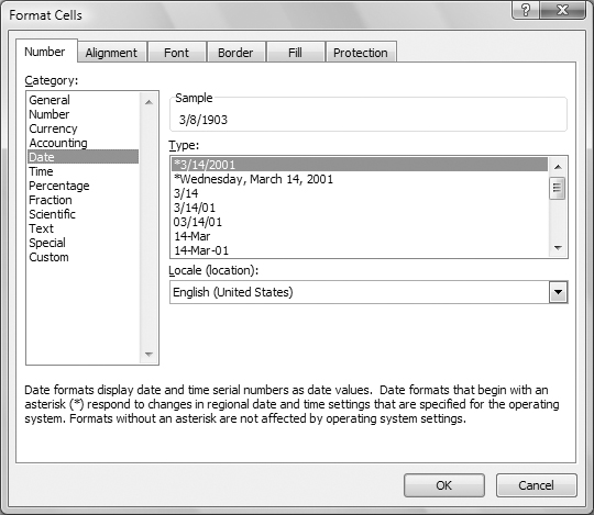
• Date formats are used to display dates.
• Time formats are used to display times.
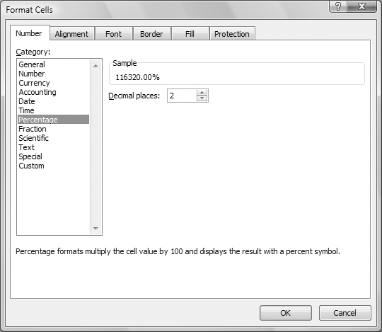
• Percentage formats are used to display percentages.
• Fraction formats are used to display decimal values as fractions.
• Scientific format is used to display values in scientific notation.
• Text format is used to display cell contents as text, the way it was entered.
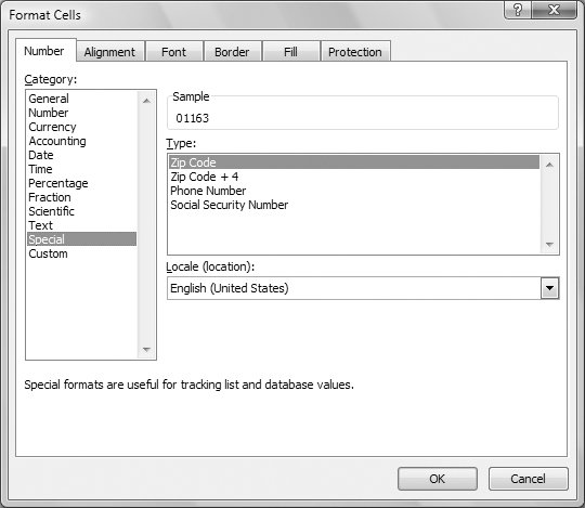
• Special formats include a variety of special purpose formatting options.
• Custom lets you create your own number format using formatting codes.
You can change number formatting of selected cells with options in the Number group of the Ribbon’s Home tab (Figure 5) or in the Number tab of the Format Cells dialog (Figures 10 through 17).
• If the integer part of a number is longer than the width of the cell or 11 digits, General number format displays it in scientific notation (Figure 3).
• Number formatting changes only the appearance of a number. Although formatting may remove decimal places from displayed numbers, it does not round numbers. Figure 4 illustrates this. Use the ROUND function, which I discuss in Chapter 5, to round numbers in formulas.
Figure 4. The two columns contain identical values, but the column on the right is formatted with the Accounting Number Format style. Because Excel performs calculations with the numbers underlying any formatting, the total on the right appears incorrect!

Figure 5. The Number group of the Ribbon’s Home tab includes commands for applying number formatting options.

• If you include characters such as dollar signs or percent symbols with a number you enter, Excel automatically assigns an appropriate built-in format to the cell.
To apply number formatting with Number group options
To apply one of the predefined number formats, choose an option from the Number Format drop-down list (Figure 6) or click the button for the format you want to apply (Figure 5):
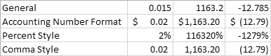
• Accounting Number Format displays the number as currency, with a currency symbol, commas, and two decimal places.
• Percent Style displays the number as a percentage with a percent symbol and two decimal places.
• Comma Style displays the number with a comma and two decimal places.
Figure 6. The Number Format drop-down list offers several predefined number formats.

Figure 7 shows examples of some of these formats.
Figure 7. Three different values, each with one of the Number group’s number formats applied.
• The Accounting Number Format button is also a menu. Click the triangle on the button to choose from additional options (Figure 8).
Figure 8. The Accounting Number Format button is also a menu.

To change the number of decimal places
Click one of the Decimal buttons in the Number group of the Ribbon’s Home tab (Figure 5):
• Increase Decimal displays an additional decimal digit.
• Decrease Decimal displays one less decimal digit.
To apply number formatting with the Format Cells dialog
1. Choose Home > Cells > Format > Format Cells (Figure 9), press ![]() , or click the dialog box launcher button in the lower-right corner of the Number group (Figure 5).
, or click the dialog box launcher button in the lower-right corner of the Number group (Figure 5).
Figure 9. The Format menu offers access to many of the formatting commands discussed in this chapter.

2. If necessary, in the Format Cells dialog that appears, click the Number tab to display its options (Figure 10).
3. Choose a number format category from the Category list.
4. Set options in the dialog. The options vary for each category; Figures 10 through 17 show examples. Check the Sample area to see the number in the active cell with the formatting options you selected applied.
Figures 10 & 11. Examples of options in the Number tab of the Format Cells dialog.

Figures 12, 13, 14, 15, 16, & 17. More examples of options in the Number tab of the Format Cells dialog.


Alignment
Excel offers a wide variety of options to set the way characters are positioned within a cell (Figure 18):
• Text Alignment options position the text within the cell.
• Orientation options control the angle at which text appears within the cell.
• Text Control options control how text appears within the cell.
• Right-to-left options control the reading order of cell contents. This option is useful for languages that read characters from right-to-left rather than left-to-right.
Figure 18. Examples of cells with different alignment options applied.

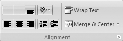
You can change alignment settings for selected cells with the Alignment group of the Ribbon’s Home tab (Figure 19) or the Alignment tab of the Format Cells dialog (Figure 21).
Figure 19. The Alignment group of the Ribbon’s Home tab offers a number of alignment options.
• By default, within each cell, Excel left aligns text and right aligns numbers. This is called General alignment.
• Although it’s common to center headings over columns containing numbers, the work-sheet may actually look better with headings right aligned. Figure 20 shows an example.
Figure 20. Headings sometimes look better when they’re right aligned (right) rather than centered (left) over columns of numbers.

• The Merge & Center option for text control is handy for centering worksheet titles over the cells in use.
To set text alignment with Alignment group options
1. To set vertical alignment, click the Alignment group button for the type of alignment you want to apply (Figure 19):
• Top align aligns cell contents against the top of the cell.
• Middle align centers cell contents between the top and bottom of the cell.
• Bottom align aligns cell contents against the bottom of the cell.
2. To set horizontal alignment, click the Alignment group button for the type of alignment you want to apply (Figure 19):
• Align Left aligns cell contents against the left side of the cell.
• Center centers cell contents between the left and right sides of the cell.
• Align Right aligns cell contents against the right side of the cell.
To set text alignment with the Format Cells dialog
1. Choose Home > Cells > Format > Format Cells (Figure 9), press ![]() , or click the dialog box launcher button in the lower-right corner of the Alignment group (Figure 19).
, or click the dialog box launcher button in the lower-right corner of the Alignment group (Figure 19).
2. The Format Cells dialog appears. If necessary, click the Alignment tab to display its options (Figure 21).
Figure 21. The Alignment tab of the Format cells dialog.

3. To set horizontal text alignment, choose an option from the Horizontal drop-down list (Figure 22):
• General applies default alignment.
• Left (Indent) aligns cell contents against the left side of the cell. It also allows you to indent cell contents.
• Center centers cell contents between the left and right sides of the cell.
• Right (Indent) aligns cell contents against the right side of the cell.
• Fill repeats the cell contents to fill the cell.
• Justify stretches multiple lines of text across the cell so all lines except the last fill the cell from left to right.
• Center Across Selection centers the active cell’s contents across the selected cells.
• Distributed (Indent) distributes the cell’s contents horizontally within the cell.
Figure 22. Options on the Horizontal drop-down list.

4. To set vertical text alignment, choose an option from the Vertical drop-down list (Figure 23):
• Top aligns cell contents against the top of the cell.
• Center centers cell contents between the top and bottom of the cell.
• Bottom aligns cell contents against the bottom of the cell.
• Justify stretches multiple lines of text from the top to the bottom of the cell.
• Distributed distributes the cell’s contents vertically within the cell.
Figure 23. Options on the Vertical drop-down list.

5. Click OK.
To indent cell contents with Alignment group options
Click the Alignment group button for the indentation change you want:
• Decrease Indent decreases the amount of indentation.
• Increase Indent increases the amount of indentation (Figure 24).
Figure 24. This cell’s contents were indented by clicking the Increase Indent button twice.
![]()
To indent cell contents with the Format Cells dialog
1. Choose Home > Cells > Format > Format Cells (Figure 9), press ![]() , or click the dialog box launcher button in the lower-right corner of the Alignment group (Figure 19).
, or click the dialog box launcher button in the lower-right corner of the Alignment group (Figure 19).
2. In the Format Cells dialog that appears, click the Alignment tab to display its options (Figure 21).
3. Choose Left (Indent) from the Horizontal drop-down list (Figure 25).
Figure 25. To indent text, set Text alignment options like this.
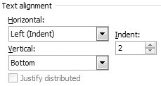
4. In the Indent text box, enter the number of characters by which you want to indent cell contents (Figure 25).
5. Click OK.
To wrap text with Alignment group options
Click the Wrap text button to enable text wrapping within a cell (Figure 19).
To set text control options with the Format Cells dialog
1. Choose Home > Cells > Format > Format Cells (Figure 9), press ![]() , or click the dialog box launcher button in the lower-right corner of the Alignment group (Figure 19).
, or click the dialog box launcher button in the lower-right corner of the Alignment group (Figure 19).
2. In the Format Cells dialog that appears, click the Alignment tab to display its options (Figure 21).
3. Turn on any valid combination of the check boxes in the Text control area.
4. Click OK.
• As shown in Figures 26 through 28, the Wrap text and Shrink to fit options can be used to fit cell contents within a cell.
Figure 26. Select a cell with too much information.
![]()
Figure 27. Here’s the cell from Figure 26 with Wrap text applied.
![]()
Figure 28. Here’s the cell from Figure 26 with Shrink to fit applied.
![]()
To merge & center cells with Alignment group options
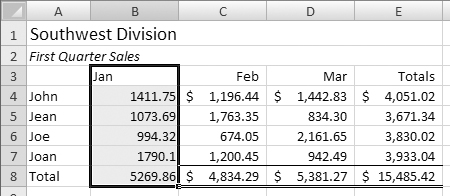
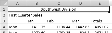
1. Select the cell(s) whose contents you want to center, along with the cells of the columns to the right that you want to center across (Figure 29).
Figure 29. Select the cells you want to merge and center.

2. Click the Merge & Center button on the Alignment group of the Ribbon’s Home tab. The cell contents shift so they’re centered between the left and right sides of the selected area (Figure 30).
Figure 30. The cells are merged together and the cell contents are centered in the merged cell.
• The Merge & Center button is also a menu. Click its triangle to choose from other options (Figure 31), each of which is illustrated in Figure 32.
Figure 31. The Merge & Center button is also a menu with related options.
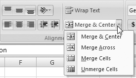
Figure 32. The Merge & Center button menu’s options, illustrated.

To merge & center cells with the Format Cells dialog
1. Select the cell(s) whose contents you want to center, along with the cells of the columns to the right that you want to center across (Figure 29).
2. Choose Home > Cells > Format > Format Cells (Figure 9), press ![]() , or click the dialog box launcher button in the lower-right corner of the Alignment group (Figure 19).
, or click the dialog box launcher button in the lower-right corner of the Alignment group (Figure 19).
3. In the Format Cells dialog that appears, click the Alignment tab to display its options (Figure 21).
4. Choose Center from the Horizontal drop-down list (Figure 22).
5. Turn on the Merge cells check box.
6. Click OK. The cell contents shift so they’re centered between the left and right sides of the selected area (Figure 30).
• You can get similar results by choosing Center Across Selection from the Horizontal drop-down list (Figure 22) in step 4 and skipping step 5. The cells, however, are not merged, so an entry into one of the adjacent cells could obscure the centered contents.
To change cell orientation with Alignment group options
Choose an option from the Orientation button’s menu (Figure 33). Figure 34 shows examples of each of the options.
Figure 33. The Orientation button is a menu with various orientation options.

Figure 34. You can achieve a variety of orientation effects.
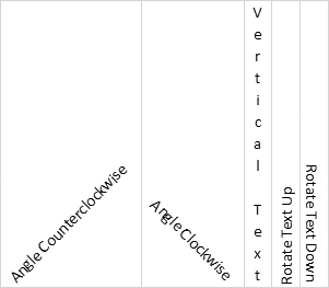
• Rotated text appears better when printed than it does on screen (Figure 34).
• Changing the orientation of a cell’s contents can change the height and width of the cell’s row (Figure 34).
To change cell orientation with the Format Cells dialog
1. Choose Home > Cells > Format > Format Cells (Figure 9), press ![]() , or click the dialog box launcher button in the lower-right corner of the Alignment group (Figure 19).
, or click the dialog box launcher button in the lower-right corner of the Alignment group (Figure 19).
2. In the Format Cells dialog that appears, click the Alignment tab to display its options (Figure 21).
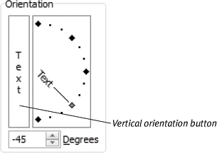
3. Set options in the Orientation area (Figure 35) using one of these methods:
• To display text characters one above the other, click the Vertical Orientation button.
• To display text characters at an angle, drag the red diamond in the rotation area or enter an angle value in the Degrees box.
Figure 35. Set options using the orientation area of the Format Cells dialog.
4. Click OK.
• You cannot set orientation options if Center Across Selection is chosen from the Horizontal drop-down list (Figure 22). Choose another option before you set orientation.
• You can enter either a positive or negative value in the Degrees box (Figure 35).
• Rotated text appears better when printed than it does on screen (Figure 34).
• Changing the orientation of a cell’s contents can change the height and width of the cell’s row (Figure 34).
• Rotating the text in column headings often enables you to decrease column width, thus enabling you to fit more information on screen or on paper. I tell you how to change column width later in this chapter.
To change text direction
1. Choose Home > Cells > Format > Format Cells (Figure 9), press ![]() , or click the dialog box launcher button in the lower-right corner of the Alignment group (Figure 19).
, or click the dialog box launcher button in the lower-right corner of the Alignment group (Figure 19).
2. In the Format Cells dialog that appears, click the Alignment tab to display its options (Figure 21).
3. Choose an option from the Text Direction drop-down list (Figure 36):
• Context sets text direction based on the cell content’s context or language.
• Left-to-Right enables you to enter text from left to right.
• Right-to-Left enables you to enter text from right to left.
Figure 36. Use this drop-down list to set text direction options.

Font Formatting
Excel uses 11 point Calibri as the default font or typeface for worksheets. You can apply a variety of font formatting options to cells, some of which are shown in Figure 37:
• Font is the typeface used to display characters. This includes all fonts properly installed in your system.
• Font style is the weight or angle of characters. Options usually include Regular, Bold, Italic, and Bold Italic.
• Size is the size of characters, expressed in points.
• Underline is character underlining. Don’t confuse this with borders, which can be applied to the bottom of a cell, regardless of its contents.
• Color is character color.
• Effects are special effects applied to characters.
Figure 37. This example shows font, font size, and font style applied to the contents of cells.
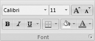
You can apply font formatting with the Font group of the Ribbon’s Home tab (Figure 38), shortcut keys, and the Format Cells dialog.
Figure 38. The Font group of the Ribbon’s Home tab.
• You can change the formatting of individual characters within a cell. Just double-click the cell to make it active, select the characters you want to change (Figure 39), and use the appropriate font formatting technique to change the characters (Figure 40).
Figure 39. You can also select individual characters within a cell ...
![]()
Figure 40. ... and apply formatting to them.
![]()
To apply font formatting with Font group options or shortcut keys
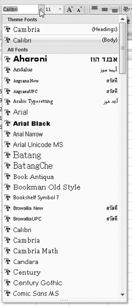
• Choose a font from the Font drop-down list (Figure 41).
Figure 41. The Font drop-down list in the Font group of the Ribbon’s Home tab lists all of the fonts installed in your system.
• Click on the Font box to select its contents, type in the name of the font you want to apply, and press ![]() .
.
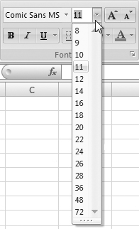
2. To change the character size:
• Choose a size from the Font Size drop-down list (Figure 42).
Figure 42. You can choose a size from the Font Size drop-down list.
• Click on the Font Size box to select its contents, type in a size, and press ![]() .
.
• Click the Increase Font Size or Decrease Font Size buttons to increment or decrement the font size by one pixel.
3. To change the character style, click any combination of font style buttons or press corresponding shortcut keys:
• Bold or ![]() makes characters appear bold.
makes characters appear bold.
• Italic or ![]() makes characters appear slanted.
makes characters appear slanted.
• Underline or ![]() applies a single underline to characters.
applies a single underline to characters.
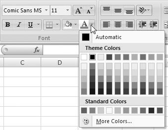
4. To change the character color, choose a color from the Font Color menu (Figure 43).
Figure 43. The Font Color menu on the Formatting toolbar enables you to apply color to characters.
• Font size must be between 1 and 409 points in half-point increments. (In case you’re wondering, 72 points equals 1 inch.)
• The Automatic color option (Figure 43) tells Excel to automatically apply color based on other formatting options.
To apply font formatting with the Format Cells dialog
1. Choose Home > Cells > Format > Format Cells (Figure 9), press ![]() , or click the dialog box launcher button in the lower-right corner of the Font group (Figure 38).
, or click the dialog box launcher button in the lower-right corner of the Font group (Figure 38).
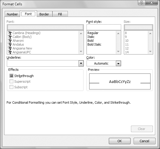
2. In the Format Cells dialog that appears, click the Font tab to display its options (Figure 44).
Figure 44. The Font tab of the Format Cells dialog.

3. Set options as desired:
• Select a font from the Font list or type a font name into the text box above the list.
• Select a style from the Font style list or type a style name into the text box above the list.
• Select a size from the Size list or type a size into the text box above the list.
• Choose an underline option from the Underline drop-down list (Figure 45).
Figure 45. Excel offers several underlining options.

• Choose a font color from the Color drop-down list (Figure 46).
Figure 46. The Color drop-down list in the Format Cells dialog.

• Turn on check boxes in the Effects area to apply font effects.
4. When the sample text in the Preview area looks just the way you want, click OK.
• To return a selection to the default font, turn on the Normal font check box in the Format Cells dialog (Figure 44).
• The accounting underline options in the Underline drop-down list (Figure 45) stretch almost the entire width of the cell.
• The Automatic color option (Figure 46) tells Excel to automatically apply color based on other formatting options.
Borders
Excel offers many border styles that you can apply to separate cells or a selection of cells (Figure 47).
Figure 47. Use borders to place lines under headings and above and below column totals.
Use the Font group of the Ribbon’s Home tab or the Format Cells dialog to add and format borders.
To add borders with the Font group’s Border button
1. Select the cell(s) you want to add borders to.
2. Choose the type of border you want to apply from the Borders menu (Figure 48).
Figure 48. The Borders menu in the Font group of the Ribbon’s Home tab.

• To remove borders from a selection, choose No Border from the Border menu (Figure 48). If the border does not disappear, it may be applied to a cell adjoining the one you selected.
• The accounting underline options on the Underline drop-down list in the Format Cells dialog (Figure 45) are not the same as borders. They do not stretch across the entire width of the cell and they only appear when the cell is not blank.
To add borders with the Format Cells dialog
1. Choose Home > Cells > Format > Format Cells (Figure 9), press ![]() , or click the dialog box launcher button in the lower-right corner of the Font group (Figure 38).
, or click the dialog box launcher button in the lower-right corner of the Font group (Figure 38).
2. In the Format Cells dialog that appears, click the Border tab to display its options (Figure 49).
Figure 49. The Border tab of the Format Cells dialog with several cells selected.

3. Select a line style in the Line area.
4. If desired, select a color from the Color drop-down list, which looks just like the one in Figure 46.
5. Set individual borders for the selected cells using one of these methods:
• Click one of the buttons in the Presets area to apply a predefined border. (None removes all borders from the selection.)
• Click a button in the Border area to add a border to the corresponding area.
• Click between the lines in the illustration in the Border area to place corresponding borders.
6. Repeat steps 3, 4, and 5 until all the desired borders for the selection are set.
7. Click OK.
• To get the borders in your worksheet to look just the way you want, be prepared to make several selections and trips to the Border tab of the Format Cells dialog.
Cell Shading
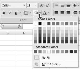
Excel’s shading feature lets you add color to cells (Figure 50), either with or without patterns. You can do this with the Fill Color menu on the Font group (Figure 51) of the Ribbon’s Home tab or in the Format Cells dialog.
Figure 50. Use Excel’s cell shading feature to add fill colors and patterns to cells.
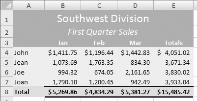
Figure 51. The Fill Color menu in the Font group of the Ribbon’s Home tab.
• By combining two colors with a pattern, you can create various colors and levels of shading.
• Be careful when adding shading to cells! If the color is too dark, cell contents may not be legible.
• To improve the legibility of cell contents in shaded cells, try making the characters bold.
• For a different look, use a dark color for the cell and make its characters white (Figure 50).
To apply shading with the Font group’s Fill Color menu
1. Select the cell(s) to which you want to apply shading.
2. Choose a color from the Fill Color menu (Figure 51).
To apply shading with the Format Cells dialog
1. Choose Home > Cells > Format > Format Cells (Figure 9), press ![]() , or click the dialog box launcher button in the lower-right corner of the Font group (Figure 38).
, or click the dialog box launcher button in the lower-right corner of the Font group (Figure 38).
2. In the Format Cells dialog that appears, click the Fill tab to display its options (Figure 52).
Figure 52. The Fill tab of the Format Cells dialog.

3. Select a color from the Background Color palette.
4. If desired, choose a foreground color from the Pattern Color drop-down list (Figure 53) and a pattern from the Pattern Style drop-down list (Figure 54).
Figure 53. Use the Pattern Color drop-down list to choose a foreground color for a patterned fill ...
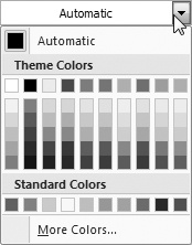
Figure 54. ... and then use the Pattern Style drop-down list to choose a pattern.

5. When the Sample area of the dialog looks just the way you want your selection to look, click OK.
• You can use the Fill Effects and More Colors button to apply a gradient or select from other background colors.
• Use fill patterns with care! If there isn’t enough contrast between cell contents and a patterned fill, the cell contents may be impossible to read.
Themes & Cell Styles
Excel includes two related features to help you apply professional-looking formatting to your worksheet files:
• Themes are collections of color-coordinated formatting options that affect the overall design of an entire worksheet (Figures 55 and 56). Excel includes 20 built-in themes, but you can find and install others from the Microsoft Office Online Web site (office.microsoft.com). You can even make changes to an existing theme and save them as a new theme.
Figure 55. An unformatted worksheet with the default Office theme applied.

Figure 56. The same worksheet shown above but with the Civic theme applied. Note the different font applied.

• Cell Styles are collections of formatting options based on the currently applied theme. Cell styles are designed for specific purposes—for example, for cells containing worksheet headings, values, or links. Cell Styles can include all formatting options discussed up to this point: number formatting, alignment, font, border, and fill. You can use the predefined cell styles or create your own.
There are three main benefits to using themes and cell styles to format your worksheets:
• They make it very quick and easy to format a worksheet.
• They ensure consistent formatting throughout a worksheet.
• They can give your worksheets a professional, polished appearance.
To use themes and cell styles
1. Choose a theme for the active worksheet (Figures 55 and 56).
2. Select one or more cells and choose a cell style to apply to the selection.
3. Repeat step 2 until you’ve applied all the styles you want to use.
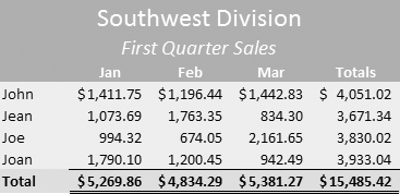
4. Apply other formatting options as desired to complete the worksheet formatting process formatting (Figure 57).
Figure 57. When you’re finished applying cell styles and other formatting options, the worksheet might look like this.
In this part of the chapter, I explain how to use the themes and cell styles features.
• It’s important to note that themes work best on worksheets with no formatting applied. Applying a different theme will not change the appearance of cells that have conflicting formatting applied. For example, if you change the font of some cells in your worksheet and then apply a different theme, the theme’s font will not be applied to those cells with the different font manually applied.
• Themes can be applied to all Microsoft Office programs—not just Excel. So you can use the same theme in Excel, Word, and PowerPoint to maintain a consistent look for all of your Microsoft Office documents.
• The themes and cell styles features are heavily dependent on color. If you plan to print your work and don’t have access to a color printer, you may want to stick to more basic formatting options.
• Once you get the hang of using Excel’s formatting options and cell styles, you may want to experiment with creating your own cell styles. This advanced feature of Excel is beyond the scope of this book, but you can find articles about it on the book’s support Web site, www.marialanger.com/excelquickstart/.
• Once you have applied cell styles to a worksheet, changing the theme simply applies different theme elements to it. Figure 58 shows how the worksheet in Figure 57 might look with another theme applied.
Figure 58. Don’t like the overall look of your formatted worksheet? No problem. Just change the theme. Here’s the same worksheet with the Paper theme applied.
To apply a theme
1. Activate the worksheet you want to apply the theme to (Figure 55).
2. Choose Page Layout > Themes > Themes to display the Theme menu (Figure 59).
Figure 59. You can find the Theme menu on the Ribbon’s Page Layout tab.

3. Click to select the theme you want to apply. The appearance of the worksheet changes to reflect the theme’s settings (Figure 56).
• Three menu commands at the bottom of the Themes menu (Figure 59) offer additional options for using themes:
• More Themes on Microsoft Office Online uses your default Web browser to display the templates page on the Microsoft Office Online Web site, which offers free themes you can download and use with Excel.
• Browse for Themes enables you to open a theme file already saved on your hard disk or a network location.
• Save Current Theme enables you to save the current theme as a new theme. Use this option if you have customized a theme and want to use the customized version again and again.
To customize a theme
1. Apply the theme you want to customize.
2. Choose an option from any combination of menus in the Themes group of the Page Layout tab (Figure 60):
• Colors (Figure 61) enables you to choose a color scheme for the theme.
• Fonts (Figure 62) enables you to choose a combination of fonts for the theme.
• Effects (Figure 63) enables you to choose a combination of lines and fill effects.
Figure 60. The Themes group on the Page Layout tab.

Figure 61. The Colors menu displays color schemes for all themes.

Figure 62. The Fonts menu lists all theme font combinations.

Figure 63. The Effects menu lets you choose from the line and fill effects combinations used by themes.

Your changes are applied immediately.
• You can create your own custom color scheme for a theme. Choose Page Layout > Themes > Colors > Create New Theme Colors (Figure 61) to get started.
• You can also create a new set of theme fonts. Choose Page Layout > Themes > Fonts > Create New Theme Fonts (Figure 62) to get started.
To apply cell styles
1. Select the cell(s) you want to apply the formatting to (Figure 64).
Figure 64. Select the cell you want to apply formatting to.
2. Choose Home > Styles > Cell Styles to display the Cell Styles menu (Figure 65).
Figure 65. The Cell Styles menu offers a wide variety of predefined styles.
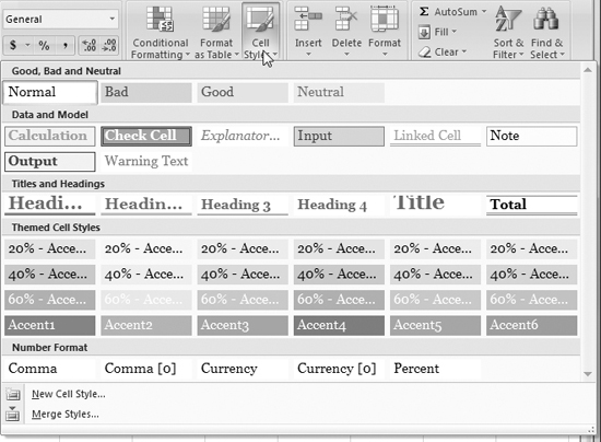
3. Click to select the style you want to apply. Styles are broken down into five different categories:
• Good, Bad and Neutral are formats you may want to apply to highlight certain cells in your worksheet.
• Data and Model are formats to indicate certain types of cell contents.
• Titles and Headings are formats for worksheet titles, column headings, and column totals.
• Themed Cell Styles are formats combining font and fill formatting that directly correspond to the currently applied theme.
• Number Format are standard, commonly used number formats.
The option you choose is immediately applied to the selected cell(s) (Figure 66).
Figure 66. Here’s the Accent1 style applied to a cell.

4. Repeat steps 1 through 3 to format the worksheet as desired.
• You can combine styles from multiple cell style categories to combine formatting effects. Some styles, however, will overwrite others.
• You can always modify the appearance of a cell with a cell style applied by manually applying other formatting options as discussed in the first half of this chapter.
• To remove all styles from a cell, choose Home > Styles > Cell Styles > Normal.
• The Cell Styles menu includes two other options you can use to work with cell styles:
• New Cell Style enables you to create a new style. Once created, it will appear at the top of the Cell Style menu.
• Merge Styles enables you to import styles from another Excel Workbook file into the current file.
Conditional Formatting
Excel’s Conditional Formatting feature enables you to set up special formatting that is automatically applied by Excel only when cell contents meet certain criteria.
For example, say you have a worksheet containing the total sales for each member of your company’s sales staff. You want to display all sales over $1,500 in bold, blue type with a light blue background and black border. You can use Conditional Formatting to automatically apply the desired formatting in cells containing values over 1,500 (Figure 67).
Figure 67. Conditional Formatting instructs Excel to format cells based on their contents.

The conditional formatting feature has been revised and improved in Excel 2007 to make it more flexible than ever before. You can now create and apply rules to a selection to determine when conditional formatting will be applied. There are six types of rules:
• Format all cells based on their values applies fill colors to cells depending on their values. For example, you can set low numbers to be orange and high values to be yellow with values in between colored with colors on a gradient.
• Format only cells that contain applies formatting to only those cells that meet certain criteria you specify.
• Format only top or bottom ranked values applies formatting to only those cells containing the highest or lowest values.
• Format only values that are above or below average applies formatting to the cells containing values that are above or below the average of all the cells, as calculated by Excel.
• Format only unique or duplicate values applies formatting to only those cells containing unique or duplicate values.
• Use a formula to determine which cells to format only formats those cells containing results that match the results of a formula you specify.
Clearly, there are many different ways you can use this feature to format worksheet contents—far too many to cover in detail in this book.
In this section, I explain how to use some basic conditional formatting options. You can apply what you learn here to other conditional formatting tasks.
To format cells with contents above a certain value
1. Select the cells you want to be considered for conditional formatting.
2. Choose Home> Styles > Conditional Formatting > Highlight Cells Rules > Greater Than (Figure 68) to display the Greater Than dialog (Figure 69).
Figure 68. The Highlight Rules submenu on the Conditional Formatting Menu.

Figure 69. The Greater Than dialog with the selected cells behind it.
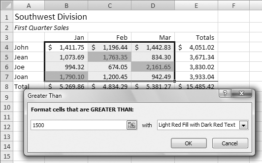
3. Enter a value in the box on the left side of the dialog. As the value changes, Excel highlights different cells in the selection (Figure 69).
4. Choose a predefined formatting option from the drop-down list in the Greater Than dialog (Figure 70).
Figure 70. Excel offers several predefined formatting options.

or
Choose Custom Format from the drop-down list in the Greater Than dialog (Figure 70), set options in the Format Cells dialog that appears (Figure 71), and click OK.
Figure 71. Use the Format Cells dialog to set up custom formatting options.
5. Click OK in the Greater Than dialog to save your settings and apply the formatting (Figure 67).
• The value that appears by default in the Greater Than dialog (Figure 69) is the average of all selected cells.
To add data bars to cells
1. Select the cells you want to be considered for conditional formatting.
2. Choose Home> Styles > Conditional Formatting > Data Bars to display a submenu of data bar colors (Figure 72) and choose a color.
Figure 72. Data Bars options for Conditional Formatting.

Data bars indicating values appear within each cell of the selection (Figure 73).
Figure 73. Data Bars are a cool way to visualize numbers, right in your worksheet.
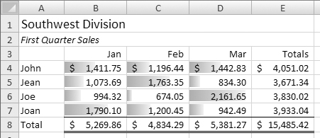
• The Color Scales and Icon Sets options offer two other ways for using color or images to indicate values in a cell. Data bars are my favorite, however, because I think they’re least intrusive and maintain the readability of cell contents.
To create a custom rule
1. Select the cells you want to be considered for conditional formatting.
2. Choose Home > Styles > Conditional Formatting > New Rule (Figure 74). The New Formatting Rule dialog appears (Figure 75).
Figure 74. The Conditional Formatting menu.

Figure 75. The New Formatting Rule dialog displaying options for the rule to format all cells based on their values.

3. Select one of the rule types in the top half of the dialog. The bottom half of the dialog changes to offer applicable options (Figure 76).
Figure 76. Selecting a different rule type displays different options.

4. Set options in the bottom half of the dialog.
5. If custom formatting is available for the rule, click the Format button. Then use the Format Cells dialog that appears (Figure 71) to set formatting options for the cells that match the criteria and click OK.
6. Click OK in the New Formatting Rule dialog to save your settings and apply the formatting.
• Two other Conditional Formatting menu options can help you work with the Conditional Formatting feature:
• Clear Rules enables you to clear conditional formatting rules from selected cells, the entire worksheet, or other groups of Excel cells.
• Manage Rules displays the Conditional Formatting Rules Manager, which enables you to create, edit, and delete conditional formatting rules.
The Format Painter
The Format Painter lets you copy cell formatting and apply it to other cells. This can help you format worksheets quickly and consistently.
To use the Format Painter
1. Select a cell with the formatting you want to copy.
2. Click Home > Clipboard > Format Painter (Figure 77). The mouse pointer turns into a little plus sign with a paintbrush beside it and a marquee appears around the original selection (Figure 78).
Figure 77. The Home tab’s Clipboard group.

Figure 78. When you click the Format Painter button, a marquee appears around the original selection and the mouse pointer turns into the Format Painter pointer.
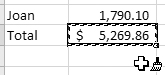
3. Use the Format Painter pointer to select the cells you want to apply the formatting to (Figure 79). When you release the mouse button, the formatting is applied (Figure 80).
Figure 79. Drag to select the cells to which you want to copy formats.

Figure 80. When you release the mouse button, the formatting is applied.

• You can double-click the Format Painter button in step 1 to continue applying a copied format throughout the worksheet. Press ![]() or click the Format Painter button again to stop applying the format and return the mouse pointer to normal.
or click the Format Painter button again to stop applying the format and return the mouse pointer to normal.
• You can also use the Clipboard group’s Copy and Paste > Paste Special commands to copy the formatting of selected cells and paste it into other cells.
Column Width & Row Height
If the data you enter into a cell doesn’t fit, you can make the column wider to accommodate all the characters. You can also make columns narrower to use worksheet space more efficiently. And although Excel automatically adjusts row height when you increase the font size of cells within the row, you can increase or decrease row height as desired.
Excel offers two ways to change column width and row height: with the mouse and with Format menu commands.
• If text typed into a cell does not fit, it appears to overlap into the cell to its right (Figure 81). Even though the text may appear to be in more than one cell, all of the text is really in the cell in which you typed it. (You can see for yourself by clicking in the cell to the right and looking at the formula bar—it will not contain any part of the text!) If the cell to the right of the text is not blank, the text appears truncated (Figure 82). Don’t let appearances fool you. The text is still all there; the missing part is just hidden by the contents of the cell beside it.
Figure 81. When text doesn’t fit in a cell, it appears to overlap into the cell beside it ...
![]()
Figure 82. ... unless the cell beside it isn’t blank.
![]()
• If a number doesn’t fit in a cell, the cell fills up with pound signs (#) (Figure 83). To display the number, make the column wider (Figure 84) or change the number formatting to omit symbols and decimal places (Figure 85). I tell you how to make columns wider on the next page and how to change number formatting earlier in this chapter.
• Setting column width or row height to 0 (zero) hides the column or row.
Figure 83. When a number doesn’t fit in a cell, the cell fills with # signs.
![]()
Figure 84. You can make the number fit by making the cell wider ...
![]()
Figure 85. ... or by changing the number’s formatting to remove decimal places.
![]()
To change column width or row height with the mouse
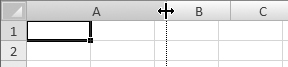
1. Position the mouse pointer on the line right after the column letter(s) (Figure 86) or right below the row number (Figure 87) of the column or row you want to change. The mouse pointer turns into a line with two arrows coming out of it.
Figure 86. Position the mouse pointer on the right border of a column heading ...

Figure 87. ... or on the bottom border of a row heading.

2. Press the mouse button and drag:
• To make a column narrower, drag to the left.
• To make a column wider, drag to the right.
• To make a row taller, drag down.
• To make a row shorter, drag up.
As you drag, a dotted line moves along with the mouse pointer (Figure 88) and the width or height of the column or row appears in a little box.
Figure 88. Drag to reposition the border, thus changing the width of the column (as shown here) or height of the row.
3. Release the mouse button. The column width or row height changes.
• When you change column width or row height, you change the width or height for the entire column or row, not just selected cells.
• To change column width or row height for more than one column or row at a time, select multiple columns or rows and drag the border of one of them. I explain how to select entire columns and rows in Chapter 2.
• If you drag a column or row border all the way to the left or all the way up, you set the column width or row height to 0, hiding the column or row from view. I tell you more about hiding columns and rows next.
• To quickly set the width or height of a column or row to fit its contents, double-click the column or row heading border. I tell you more about this AutoFit feature later in this chapter.
To change column width or row height with menu commands
1. Select the column(s) or row(s) whose width or height you want to change.
2. Choose Home > Cells > Format > Column Width or Home > Cells > Format > Row Height (Figure 9).
3. In the Column Width dialog (Figure 89) or Row Height dialog (Figure 90), enter a new value. Column width is expressed in standard font characters while row height is expressed in points.
Figures 89 & 90. The Column Width (left) and Row Height (right) dialogs.

4. Click OK to change the selected columns’ width or rows’ height.
To hide columns or rows
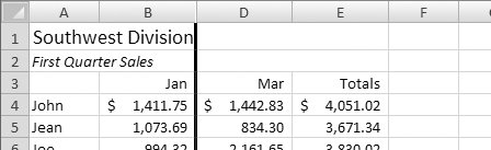
1. Select the column(s) (Figure 91) or row(s) you want to hide.
Figure 91. Select the column that you want to hide.

2. Choose Home > Cells > Format > Hide & Unhide > Hide Columns or Home > Cells > Format > Hide & Unhide > Hide Rows (Figure 92). The selected column(s) or row(s) disappear (Figure 93).
Figure 92. The Hide & Unhide submenu on the Format menu.

Figure 93. When you choose the Hide Columns command, the column disappears.
• Hiding a column or row is not the same as deleting it. Data in a hidden column or row still exists in the worksheet and can be referenced by formulas.
To unhide columns or rows
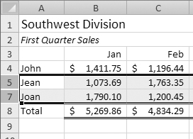
1. Select the columns or rows on both sides of the hidden column(s) or row(s) (Figure 94).
Figure 94. Select the rows above and below the hidden row.
2. Choose Home > Cells > Format > Hide & Unhide > Unhide Columns or Home > Cells > Format > Hide & Unhide > Unhide Rows (Figure 92).
The hidden column(s) or row(s) reappear (Figure 95).
Figure 95. When you choose Unhide Rows, the hidden row reappears.

AutoFit
Excel’s AutoFit feature automatically adjusts a column’s width or a row’s height so it’s only as wide or as high as it needs to be to display the information within it. This is a great way to adjust columns and rows to use worksheet space more efficiently.
To use AutoFit
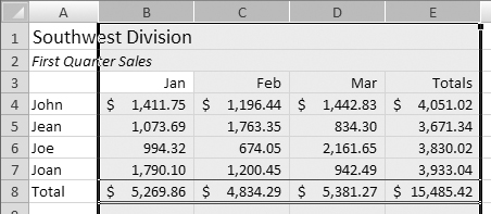
1. Select the column(s) or row(s) for which you want to change the width or height (Figure 96).
Figure 96. Select the columns for which you want to change the width.
2. Choose Home > Cells > Format > AutoFit Column Width or Home > Cells > Format > AutoFit Row Height (Figure 9).
or
Double-click on the border to the right of the column heading (Figure 86) or below the row heading (Figure 87).
The column width or row height changes to fit cell contents (Figure 97).
Figure 97. When you choose the AutoFit Column Width command, the width of the columns changes so they’re only as wide as they need to be to fit cell contents.
• To adjust a column’s width without taking every cell into consideration—for example, to exclude a cell containing a lot of text—select only the cells for which you want to adjust the column (Figure 98). When you choose Home > Cells > Format > AutoFit Column Width (Figure 9), only the cells you selected are measured for the AutoFit adjustment (Figure 99).
Figure 98. Select the cells that you want Excel to measure for the AutoFit feature.

Figure 99. When you choose the AutoFit Column Width command, Excel resizes the entire column based on the width of the contents in the selected cells.
• Use the Wrap text and AutoFit features to keep your columns narrow. I tell you about Wrap text earlier in this chapter.
Removing Formatting from Cells
You can use the Clear Formats command on the Editing Group’s Clear menu (Figure 101) to remove formatting from cells, leaving cell contents—such as values and formulas—intact.
• When you remove formats from a cell, you return font formatting to the normal font and number formatting to the General format. You also remove borders or shading added to the cell.
• Removing formatting does not affect column width or row height.
To remove formatting from cells
1. Select the cell(s) you want to remove formatting from (Figure 100).
Figure 100. Select the cells you want to remove formatting from.

2. Choose Home > Editing> Clear > Clear Formats (Figure 101). The formatting is removed but cell contents remain (Figure 102).
Figure 101. Choose Clear Formats from the Clear menu.

Figure 102. The formatting is removed but the cell contents remain.