Chapter 5. Modeling Invariants

The author believes that the notion of modeling invariants is more fundamental to MBD than translation itself. If you take away from this book a fervor for modeling invariants and never employ translation (or even the OO paradigm itself!) you will still have gained enough to significantly improve the quality of the software that you build. Your applications will be much smaller, they will be easier to understand and maintain, and they will be more reliable. That’s not incremental percentages, that’s integer factors.

Frankly, it is astonishing that the notion of modeling invariants has attracted so little attention in the literature of software engineering. For many years Steve Mellor was the only publicly visible proponent of the practice. In addition, Shlaer-Mellor and MBD are the only methodologies that explicitly integrate the practice. When presented on public forums the idea is often met with a sort of I-knew-that response that recognizes it as a good idea but assumes that everybody does it so there is no need to belabor the point. Alas, hardly anybody actually models invariants, and the best place to observe this lies in the way people partition their applications.

In Chapter 2 it was pointed out that modeling invariants was not an OO thing. One can model invariants using any software development methodology. It is simply a way of separating essential, stable structure from volatile details. However, the OO paradigm’s emphasis on abstraction, encapsulation, functional isolation, programming by contract, polymorphism, and interface boundaries is a big help in getting a handle on it.

So Just What Is Modeling Invariants?

It is about capturing invariant aspects of the problem solution in the software while relegating detailed variability to external data. Unfortunately, this tastes good but doesn’t have a lot of real meat in it. So it is time to flesh things out by providing a bit more beef.¹

As it happens, the computing space is loaded with examples of invariants. For example, 3GL languages employ invariants that are abstracted for commonly recurring themes in Turing machine programs. Things like iteration constructs and I/O calls capture basic structural invariants while handling the detailed differences in parameters embedded in the constructs. Similarly, basic aggregate data structures (array, list, etc.) provided by most languages and in libraries are simply generalized sets whose implementation is parameterized.

The computing space is also loaded with design techniques that are really examples of invariants. Perhaps the most obvious examples lie in design patterns.² Every pattern represents a generalized structure that is common across many situations and provides a mechanism for describing the differences in situations as instantiation details. Even things as disparate as coding standards and network protocols represent variations on the theme of identifying and institutionalizing invariants. So we routinely use invariants. The problem is that they are someone else’s generic invariants rather than our own problem-specific invariants.

The Invariant Side

First let’s look at the notion of invariant. As the word implies, we are talking about something that doesn’t change, something that is stable. So far, so good; nothing to boggle one’s karma. But there is a qualifying spin on this notion in the MBD context. We are talking about a particular group of invariants—those things that are stable in the customer’s problem space.

The problem space aspect is crucial because in the OO paradigm generally, and in MBD in particular, we strive to base software structure on the customer’s infrastructures. That is because we believe that the customer will adapt to change in a manner that will cause minimal disruption to existing infrastructure.³ If the software structure parallels that customer infrastructure, it should be minimally disrupted as well. And that implies maintenance with less pain.

The elegant thing about invariants is that they exist at all levels of abstraction. It is rather like a head of garlic. Around the outside there are a few big, rounded cloves. But as you peel away sheaths and cloves you find successively smaller cloves that become longer and thinner. Eventually one gets down to central cloves that are sized and shaped quite differently than the outer cloves.

The analogy is admittedly tenuous, but it underscores the point that invariants can be employed throughout the application, and that the scale and nature of those invariants will vary with the scale and context where they are applied. The big, large-scale invariants employed for application partitioning are usually pretty easy to spot. Alas, the little ones at the class and state machine level are often much tougher to recognize.

The developer must be aware that the notions of customer and problem space can be moving targets for large, complex applications, which presents problems for extracting invariants. For example, most applications have to store data persistently. It is quite common to create a subsystem to handle the actual data storage as a separate service to the rest of the application. The nature of that subsystem will depend in large measure on the nature of the persistence mechanisms (e.g., RDB versus OODB), which may be entirely transparent to the end user or customer of the software.

In such situations the customer becomes the database itself because it places constraints (requirements) upon the subsystem. The rest of the application is also a customer because of its needs (requirements) to store and access data in the database. While this changes the perspective on the subsystem’s role as a service, it shouldn’t change the fundamental abstractness of the subject matter description. That subject matter perspective provides the relevant invariants.

So for an RDB implementation of the service, the relevant invariant paradigm becomes the relational data model. While the rest of the application might think about a Clerk and the GUI subsystem may think about a Clerk Window with associated Controls, the persistence subsystem is likely to think about a Clerk Table with associated Clerk Rows instead of Clerk objects. Because the relational data model is the core paradigm, application objects need to be recast in terms of things like referential identifiers, and identity itself becomes an explicit issue. The point is that to properly model invariants one must have a deep understanding of the problem space, regardless of what that space is. As a corollary, we must also isolate and encapsulate that problem space so that we can focus on only its invariants.

In a sense, the term problem space is a bit misleading in the invariant context because we seek invariants not in the problem itself but in the environment in which the problem exists. That is, the scope of the customer domain is necessarily broader than the problem itself when looking for invariants. It is, quite literally, the entire space in which the problem lies. One view of invariants is that they are characteristics common to a set of related problems, of which the problem in hand is one. A corollary is that to recognize invariants the developer needs to practice some degree of Domain Modeling or Analysis.

The rationale for this view is that when requirements change, they will likely require that we solve a new problem that is only slightly different from the original problem. So we try to describe in software the common aspects of solutions to a set of problems and relegate the differences in those solutions to data. In general, the more broad the class of problems resolved in software, the less likely that the software will have to change over time. To put it another way, when the requirements change it becomes more likely that they will simply identify a different member of the class of problems to solve. If so, the problem is already solved generically and we only need to modify the data to reflect the new member of the problem set.

Unfortunately, it is a lot easier to describe what one does when extracting invariants than it is to describe how to do it. There aren’t a lot of cookbook guidelines because it is a relatively new technique, so the tools used in this book to describe how to do it are repetition and examples.

The Data Side

We now segue into the idea of using external data to describe detailed differences. This idea seems quite reasonable, but it begs the issue of exactly how we do that. The mechanism for converting data into different solutions is primarily based upon polymorphism, particularly parametric polymorphism. As you will recall, we use the term in the traditional software sense of obtaining different results from a generic behavior by providing different input data to the behavior.

Ad hoc polymorphism provides a clue. Those switch statements and cascaded if...else statements routinely modified behavior based upon state data. The OO paradigm simply offers an even more versatile technique through (a) extension of the notion of input parameters to all state data, particularly specification objects, and (b) dynamic instantiation of relationships to particular specification objects.

By binding instances together at runtime we get to select which state data (i.e., instance attributes) are to be used in particular circumstances. Thus, not only do we get to diddle with data values, we can also diddle with which sets of parameters to use. In particular, OO relationships tend to be instantiated based on a context that spans individual collaborations, so the relationship may be instantiated long before a particular collaboration method’s invocation. More important, that context may be defined by someone other than the client in the collaboration. It would be getting ahead of the story to go into this in greater detail here, but have faith that this is really a very powerful technique that was pretty much unavailable before the OO paradigm.

Unfortunately, some magic is required to do invariants properly. It requires a different way of thinking about problems. Of all the activities of software development, identifying invariants depends most on the experience, judgment, and skill of the developer. The good news is that it is a very learnable skill. The only innate skill required is the ability to think abstractly, which is necessary to do OO development at all. It is also one of the essential things that separates Homo sapiens from all the rest so if you can’t think abstractly, blame it on your parents.

There are no cookbook rules for doing it, so we will be spending a fair amount of time on examples, analysis patterns, and some (very loose) guidelines. But in the end you will have to rely on the time-honored paradigm of practice, practice, practice.

The Rewards

Because identifying invariants requires a lot of practice, it is important to understand why it is worth the effort. A major benefit of emphasizing invariants lies in maintainability of the application. External data is usually a lot easier to change reliably than application code because the side effects tend to be much more limited. As you may recall from the discussion of coupling in Chapter 2, data tends to be much more benign as far as dependencies go. We can misuse data, but it doesn’t actually do anything by itself. In addition, data is often easier to change because it is so narrowly defined and simple. The context for changing it is usually very well focused, and we are modifying values rather than complex syntax. We can also provide tools that make the data updates more user friendly by automating tedious activities, such as finding the right data to change.

Nearly as important, though, is the impact on the development processes. When changes are done in data the software is unaffected. No code walking. No check-in and check-out of a flock of modules. No build cycle. No software configuration management. (There is configuration management of the data, but that is usually trivial compared to software configuration management.) And there is complete confidence that if anything breaks during testing, the problem lies in the data changes because the code wasn’t touched.

What this often means is that the customers can manage the changes directly once you give them the proper tools. Usually this is nothing more than what they are already doing in some form anyway. They have to tell you what the change is, and that will very often involve specific data or identity. When you encode invariants you need to figure out how to express differences in data, and that data will necessarily be expressed in problem space terms. If it is in problem space terms, the user should be aware of it when the requirements change and use that same data to specify the requirements change. In effect, you have then moved requirements change management from executable program statements to a data entry problem in the customer’s domain.⁴

But the most important benefit to maintainability is related to application partitioning. When system partitions are defined in terms of invariant and cohesive problem space structures it brings long-term stability to the system. When those partitions are encapsulated behind disciplined interfaces we have “firewall” protection against one partition doing rude things to another. And when those partitions are cohesive and are linked by client/service relationships, the scope of requirements changes tends to be contained. That is, you tend to have to touch a lot less stuff to effect the change.

A related benefit lies in large-scale reuse. MBD focuses on large-scale reuse rather than object-level reuse. Mechanically, MBD supports large-scale reuse through things like interface discipline. But the key to any reuse lies in defining semantics for the reuse subject matter that will stand the test of time. That is, reused elements could end up being reused in situations that were undreamed of by the original developers.

That requires a high degree of cohesion and well-defined subject matter boundaries. Since reuse is ultimately driven by the customer (i.e., the customer will trigger the requirements for those undreamed of reuse situations), the cohesion and boundaries must be stable in the customer’s domain. To find that sort of stability in the customer’s domain we must look for invariants in the customer space that define both the subject matter and its boundaries. If you do that, you will have a solid basis for long-term, large-scale reuse.

Another major benefit is reduced code size. Moving details out of the software and into external data simplifies the software. In effect we are moving a ton of if...else decision making into the external data. That leaves us with simpler code. It is not uncommon for code size to be reduced by integer factors when applying invariants.

A very important corollary of reducing code size is greater reliability. Generally, the number of defects is linearly related to code size over broad intervals. So if we reduce code size, we tend to reduce the total defects in the product as well. But what about defects in the data? Well, yes, one has to add those back in. However, there are several mitigating factors:

• Data is more regularly organized (e.g., tabular values), which makes it easier to change and less error prone.

• One only has to get values right, not complex syntax (e.g., in C using “=” instead of “==” in a conditional expression).

• Context is more focused because the semantics of the data values is narrowly defined, limiting the types of errors possible.

• Data has very limited intrinsic side effects.

• The data that supports invariants will be known in the problem space, so it will be easier to validate its correctness with the customer.

• The software uses all data of a given type exactly the same way (i.e., generically).

• Data can be formatted to reduce certain types of errors.

• Tools can remove tedious tasks and provide error checking.

• Configuration data are essentially system inputs, and errors in system inputs are almost always immediately manifested as incorrect results.

• Test cases can be automatically generated from the data to reduce the likelihood of escapes.

As a general assertion it is fair to say that errors in external data are less frequent than software errors (assuming we take some elementary formatting and documentation precautions), and when they do occur they are more readily found.

In the interest of truth in advertising, it should be pointed out that most of the code size benefits are realized at the class level when implementing individual subsystems. Nonetheless, applying invariants at the application partition level does have some indirect size reduction consequences. One way this happens is through cohesion. When a partition is highly cohesive, the abstractions needed to implement it tend to be rather simple, and the partition is more easily implemented. If the subsystems are each more easily implemented, it is likely that the application will be smaller. This is because complexity breeds interaction, so with reduced complexity there tends to be less interaction and exception handling.

Examples

As indicated previously, the best way to understand the use of invariants is by example and by practice. The more exposure we have to right thinking, the better off we will be. Unfortunately, we haven’t shown enough of MBD to get into too many details, so the examples used here are rather superficial. The intent is simply to show the kind of thinking that is involved and how varied that thinking can be.

Bank ATM Software

This one has been used so many times in the literature that it has chestnut status. It is used here because a surprising number of authors have screwed it up royally by making a very elementary error in application partitioning. They made that error because they did not look carefully for problem space invariants. Figure 5-1 provides a hypothetical but plausible overall context for ATM software.

Figure 5-1. Plausible subsystems for a banking application

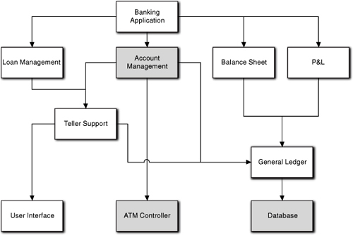
At this point we are only interested in three subsystems: Account Management, ATM Controller, and Database. Of those, we will focus primarily on the ATM Controller for this example. Basically these subsystem responsibilities can be broadly defined as follows.

Account Management. This subsystem handles the basic business processing around individual customer accounts like checking, savings, overdraft, and so forth. It is responsible for creating and deleting accounts, debiting and crediting accounts, and mundane accounting tasks like providing audit trail data.

ATM Controller. This subsystem is the software that actually controls the hardware in an ATM machine (e.g., keyboard, screen, card reader, cash dispenser, and deposit shredder). It talks to the rest of the bank’s software over a network connection.

Database. This subsystem handles persistence. Basically, it stores all the account data, audit trail logs, and other permanent data. Typically this is some big, honking enterprise database with fourteen levels of redundancy and whatnot, including some direct link to a vault at an undisclosed location under the Rocky Mountains.

So far this seems like a quite plausible partitioning of the bank’s software systems. Anyone familiar with banking systems would have little difficulty in identifying what these subsystems are about. Unless they were in the bank’s IT division, they might not know what a relational data model is, but they would have a real good idea of what data needed to be saved and how important it was.

The problem here is not with what partitions are identified. It is with the way some authors designed them. Too many ATM Controller subsystems are designed with classes like Checking Account. In one, the ATM Controller subsystem was reading and writing data directly from the Database (i.e., it was generating SQL queries and sending them off through the network port). If software engineers were certified, doing things like this should be grounds for revoking their certification and assigning them to relatively harmless tasks like formatting printed reports or creating web pages.

A class like Checking Account belongs in Account Management because that’s what that subsystem is about. But look at the description of ATM Controller. It is interested in hardware. It knows hardware. It probably even likes hardware. Hardware is enough for it to worry about, especially when every mid-level hoodlum in the country is trying to figure out a way of breaking into the ATM.

The ATM Controller subsystem talks to some entity on the other side of a network connection. The bank it is talking to may not even be the same bank that owns the ATM and installed the software! So why would the ATM Controller subsystem want to know anything at all about accounts, especially a particular bank’s accounts? The only concept it needs to share with Account Management is the notion of Message, a message identifier and the format of a packet of data tied to that identifier.

It isn’t the ATM Controller’s job to figure out if the user’s account has enough balance to cover a withdrawal, apply overdraft policy, or any of the rest of that banking business. When the user requests a withdrawal, the ATM Controller should just forward that request to the Account Management subsystem and let it figure it out. When the Account Management subsystem decides it is OK to dispense cash, it sends a message back to the ATM Controller, which then talks to the cash dispenser hardware.

And the idea of the ATM Controller dealing directly with the Database is utterly preposterous. Consider how ecstatic the bank’s DBA is going to be at the prospect of a customer remotely accessing enterprise DB objects directly from another bank’s ATM through a 56Kb modem link. Also, do you really want exactly the same code for managing two-phase commit transactions in the ATM Controller and in the software for a real bank teller terminal? But it never should get to those sorts of implementation issues. If the ATM Controller has no need to understand the semantics of Checking Account, it certainly shouldn’t know what part of that information should be persistent and what sorts of persistence mechanisms need to be used to ensure synchronization with the bank’s General Ledger. The ATM Controller should not even know that the Database exists!

So where did these guys go wrong? The main problem is bleeding cohesion across subsystems. The cohesion problem is a direct result of not looking at the invariants of the ATM Controller subsystem. There are entities common to all ATMs, like the Keyboard and Card Reader. In addition, there are things common to most hardware control systems, like registers and interrupts. Moreover, the ATM Controller software is physically separated from the rest of the software by a distributed network boundary, which screams for simple, asynchronous data messages and separation of concerns across that boundary.

Taking these things together, they strongly suggest a focus on hardware control alone. By identifying general entities common to ATM control in particular and hardware control in general, the tentative abstractions identified are clearly quite different in nature than those in Account Management. A sense of quite different concerns for the two subsystems becomes apparent.

But the most important insight into invariants lies in realizing what the ATM Controller is really about. There is a set of concrete hardware entities—card reader, display, keypad, cash dispenser, deposit shredder, and network port—that the controller must deal with. How does it deal with these entities? It reads information from and writes information to their registers. In fact, it does virtually nothing except provide an order for transferring information among the various hardware entities’ registers. What is the magic word we use in the OO paradigm for communicating between entities?

Message! The ATM Controller is about managing message flows. All it does is convert from one message format to another and ship messages around in a particular order. If it gets a message of type X from over here, it knows it should format a message of type Y and send it over there. To do that, it needs to know nothing about the semantics of the message content (i.e., what a Checking Account is). All it needs to know is what to do for each message type, and the mechanics of packing and unpacking each message type’s data format.

The invariant behavior that we need to capture in the ATM Controller software is that of a message broker. If we raise the level of abstraction of the ATM Controller to this level we accomplish a great deal. First, let’s look at the hardware side. Typically each hardware component of an ATM is manufactured by a different company and, competition being the backbone of a market-based economy, there can be multiple possible sources for each one. Does our ATM Controller software care?

Not a whole lot. We can easily describe the differences in components in configuration data. For example, the cash dispenser has to deal with a Dispense message that carries an amount. Typically the value is written to one or more registers and then there is another write to a separate register to tell the hardware to process the value. The number of registers and their addresses will probably vary from one manufacturer to another. Also, there are likely to be small differences in the way values are encoded to the registers (e.g., scaling, bit field sizes, etc.). But those differences can easily be described in data that specifies the number of registers, their addresses, their bit size, their endian, scaling rules, and any odd bit field formatting.

That data can be used to initialize an instance of a Cash Dispenser class. The Cash Dispenser will have a method, Dispense, for dispensing cash that will use the attribute values as parameters as it executes a generic routine to write the amount and trigger the cash dispensing. (We’ll see a more specific example of how to do this shortly.) At this level a cash dispenser is not that complicated, so it will only require a modest amount of cleverness to design a Dispense method that will work for any cash dispenser on the planet—and probably any in our arm of the Milky Way galaxy—provided the right external configuration data is provided.

But what about the semantics of the messages? Can that really be abstracted so readily? Yes, Grasshopper, it certainly can within the limits of today’s banking practices. There are not a lot of things the ATM’s components can do, and those are pretty well standardized in terms of banking transactions. All the heavy lifting can be done on the other side of the network port by Account Management and Database based on ATM Controller’s announcements about its user’s limited suite of activities.

In reality, an ATM Controller as proposed can be much more versatile. Suppose the bank decides to let the customer refinance a mortgage through the ATM. To do that, all we need is an additional suite of messages among display, keypad, and network port. The heavy lifting of loan approval, and so forth, will still get done on the other side of the network port. Clearly, message types, their data packet formats, and their destinations can be defined in external data fairly easily for something as simple as an ATM. With a little bit more creativity we can define message sequences (e.g., “If I receive message type A, I must send message type B”) in terms of external configuration data because in an ATM those sequences aren’t very complicated.

We can’t go into detail here (though we will later) because we need more pieces of the puzzle first. However, defining the rules for dispatching messages for an ATM Controller in data is almost trivial. Basically this means that the bank can let the customer perform almost any financial activity with the bank without touching the ATM Controller software. All the new messages, display texts, and customer keypad responses can be defined through external configuration data. This is possible because the invariant paradigm of message broker does not depend upon understanding the semantics of message content any more than an e-mail program cares about the flaming in the message body.

If you are at all familiar with hardware control systems you will no doubt have realized that this paradigm potentially has much wider scope than just ATMs. We could develop the ATM Controller software in a fashion such that it could control a wide variety of hardware systems without changing anything except the configuration data. In fact, a much better name for the subsystem might be Hardware Message Broker. If you are beginning to suspect that this notion of modeling invariants brings new meaning to the word reuse, you would be right.

In addition to better cohesion, this train of thought leads to a better perspective on the nature of the subsystem boundaries. The network provides a very natural boundary, and the characteristics of network communications color the view of inter-subsystem communications. When combined with disparate concerns on either side, the boundary becomes more than simply a technical issue for efficient transmissions.

The boundary becomes an almost conceptual separation. On one side we have hardware and bank customers; on the other side we have banking and accountants. These are entirely different concerns and views, so the network interface becomes a medium of translating from one view to the other. When we consider the possibility of the ATM belonging to a different bank, it becomes even more desirable to minimize shared views; the least common denominator representation becomes attractive. In that context there is no need to pass objects across the boundary; we convert abstractions and minimize shared views through pure message interfaces that captures only the fundamental nature of the service invariants.

The point in the last couple of paragraphs is that this view of invariants is less about general rules and policies than about defining what subject matters are. The real insight here is understanding what the subject matter should know and do. We do that by seeking out its fundamental nature. Thus, the invariant in this example is what the intrinsic nature of an ATM Controller is. Once we grasp that, the generalization to classes of problems beyond ATMs becomes clear.

Hardware Interface

In the previous example we identified an ATM Controller as being concerned with managing hardware. However, that was the megathinker view of hardware communications. In this example we will deal with hardware communications at a much lower level of abstraction.

At a high level of abstraction we can think of all hardware interfaces in terms of reading and writing hardware registers. That’s because almost all hardware provides an interface to software that is based upon the models for digital computation. We write values to registers, tell the hardware to read them, and read back values from registers when the hardware is done doing its thing (which it will announce by putting a value in a register to be read by the software).

For those of you who are not R-T/E people, the hardware guys provide the specification of the register semantics in what are known as bit sheets. The bit sheets identify registers by address, identify fields within the register {start bit, length} with a mnemonic, and provide a very brief and often unintelligible description of the field semantics. Registers usually have a fixed length in terms of bits. Things are complicated because values may not fit in a register, or fields may be split across registers, so reading or writing a single value often involves reads or writes of multiple registers. Finally, because multiple fields might be in a single register, one has to preserve the other fields’ values when writing a value to a single field. (The R-T/E people refer to this as Read/Modify/Write⁵ because we need to write the whole register. So we read the register, update just the embedded field, and then write the register.) The R-T/E people then build device drivers to run the hardware by talking to those registers.

A big problem that R-T/E software developers face is that the hardware guys are constantly changing the bit sheets as they do Engineering Change Orders (ECOs), or provide new and better circuit boards to do the same job, or simply to pull the chains of the software people. Because hardware real estate on circuit boards is precious, the hardware guys often move registers and redefine fields so they can fit everything on the circuit board with feasible artwork.⁶ So the bit sheets may be vastly different for two circuit boards that provide exactly the same functionality. Now the poor software guy trying to provide basic functionality for something like a cell phone finds that even though the phone works exactly the same way, the device driver needs to be rewritten because the bit sheets changed for a new card.

Historically, the R-T/E people actually pioneered modularity for exactly this reason. They provided a layer that would talk to the registers and provided a more generic interface to the rest of the software for the layer. Then all they had to do was replace that layer when the bit sheets changed. Today, though, we have a much better way to handle this problem so that we don’t need to touch the layer at all.

But to reach that solution we need to think about the invariants of reading and writing hardware registers. We got halfway there earlier when we said that hardware control was about reading and writing registers. We read or write exactly one register at a time. We also read or write one problem data value at a time. Hence the basic problem is to put a single data value into one or more registers, and unless one is computing a gazillion decimal places for pi, the data value is going to fit into at most three registers.

In addition, we discussed how bit sheets provide a mapping between values and register fields. Here we are interested in the invariants of mapping values into defined fields in one or more registers. If you review the paragraph that described bit sheets, you will recognize that these things are always true:

• Registers are identified by addresses.

• Registers have fixed length in bits.

• Registers have one or more fields defined in terms of {start bit, bit length}.

• Fields have a designated identity represented by a mnemonic for the value that they store.

• Values may be split across fields in different registers. (The bit sheet will specify which field in which register has the lower order bits.)

• If a register has multiple fields, one may need a Read/Modify/Write operation to set the value of a single field.

• If a value to be read or written is normally represented in more bits than the register field for it in the hardware, the value will need to be scaled.⁷

While reading and writing hardware registers is complicated, the list of possible processing activities is actually pretty short. Even better, those operations are so common that any R-T/E person can write them for a given value without much thought and possibly even when comatose. Better yet, the operations are easily separated and ordered sequentially. Thus, scaling a value to a field size is quite different than a Read/Modify/Write, and it will be done first. Best of all, the rules for those operations can be expressed exclusively in terms of bit sheet field specifications that are simply data.

That enables us to change the way we think about bit sheets. Instead of defining register fields, we can think of them as defining how individual semantic values are mapped into hardware registers. All we have to do is group together the bit sheet field specifications for the mnemonic corresponding to the value we want to read/ write, and we can “walk” those specifications in order to perform the relevant register reads and writes. And we can do that with very generic code that is parameterized with the bit sheet field definition values. A simplistic model for doing this is shown in Figure 5-2.

Figure 5-2. Invariants of low-level hardware control

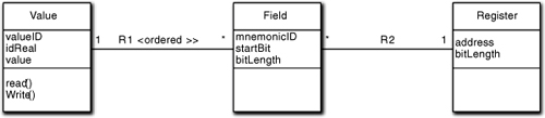
The R1 relationship is ordered based on the bit sheet values so that one can split the Value over multiple fields in the proper sequence. R1 collects only the Fields that are relevant for the Value in hand. R2 then relates each Field to the Register containing it.

Value.read() and Value.write() are generic functions that know how to convert Value.value into one or more register reads or writes. They do that by navigating R1 and R2 to get the configuration information. For example, the Write() method will check if the bit length of the Field is less than that of the containing Register and, if so, will use a Read/Modify/Write. While the method code might be a tad convoluted, you can see that the method can determine everything it needs to know from navigating the relationships. So those generic methods capture the invariants of reading and writing registers and they are parameterized by the bit sheet data. (Recall the discussion of specification objects for parametric polymorphism; Register and Field are effectively specification objects.)

From an implementation standpoint the only trickiness here lies in getting the right bit sheet information. The values of the Register and Field objects are straight out of the bit sheet specifications. Since the registers and fields are fixed in the hardware, those objects can be instantiated at start-up from external configuration data (i.e., bit sheet data). The interesting part lies in instantiating the R1 and R2 relationships for a particular Value.

R2 is already fixed by the hardware as defined in the bit sheets, so we need to map a Value to its corresponding fields in the hardware registers. To do that we map valueID into the Field’s mnemonicID, which can be provided through table lookups. Those lookup tables are instantiated from the configuration data as well.

The beauty of encoding invariants while relegating details to data in this case is manifested when the hardware guys change the bit sheets. All that changes are the data values in the configuration data; not a line of application code is changed. Better yet, we can reuse this layer across different device drivers; we just need to provide different configuration data.

The author helped develop a large device driver this way. The hardware had dozens of different cards, each with hundreds of registers. Over the life of that system dozens of new cards were introduced and there were hundreds of hardware ECOs. The device driver itself had over 250 KNCLOC of code. It was originally done procedurally without invariants. When we wrote it from scratch in an OO fashion we used invariants by putting the bit sheets in an Excel spreadsheet.⁸ The software read the spreadsheet to initialize the specification objects and the lookup tables for relationship instantiation. The interesting data point was the change in maintenance effort. The old system required eight (8) full-time people to maintain it. The new version with exactly the same functionality required one (1) person half time for maintenance.

Caveat. Our version of the example model was somewhat more complicated than the one here because we addressed things like acquiring the configuration data and instantiation. There are also more elegant ways to capture the invariants than employed here, so consider this example a simplified version to make the point about invariants rather than an actual solution to communicating with the hardware.

Note that this represents a very different view of invariants than the ATM example. In the ATM example we used invariants to formalize our view of the essence of a subject matter; that is, the invariants described what the subject matter actually was. That, in turn guided how we abstracted the problem space. In this example, the invariants are basically a set of well-defined rules for converting the value view to the register view. Those rules would be readily recognized by any R-T/E developer as basic technique. Thus the tricky part was recasting some of those rules in terms of data and static relationship structure.

Depreciation

The notion of amortized depreciation is relevant to all commercial businesses. It is also a classic example of failing to recognize invariants because it is almost never implemented with them. The basic notion is simple. For accounting and tax purposes, assets are depreciated for a fixed number of years according to a specific formula based upon a base value of the asset at the time of its acquisition. Different formulas can be used for different types of assets. The business can often select the formula to use for a particular type of assets from a fixed set of choices. The rules governing how depreciation is applied are defined by organizations like the IRS and FASB. The most obvious solution is shown in Figure 5-3.

Figure 5-3. Model for depreciation wholly contained in a single class

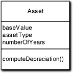
We have an Asset class with a computeDepreciation behavior and attributes for baseValue, assetType, and numberOfYears. The computeDepreciation method implements the particular formula that the bean counters have deemed appropriate for this type of asset. So far, so good, except for a few niggling details.

• The formula in computeDepreciation is hard-coded in the method, so if the formula changes we must modify the implementation of Asset.

• Assets with different types may use different formulas, which means we need some sort of substitution of the formula with assetType.

• The notion of asset type may have other uses orthogonal to depreciation for describing what the asset actually is. This leads to a proliferation of combinatorial values for assetType.

• The powers that be regularly change the rules about what formulas and time duration can be used.

• The bean counters periodically exercise their option to change the formula and/ or duration for particular assets.

• The bean counters periodically add new assets with new types or change the types of existing assets.

Dealing with all that in a single method tends to get a bit clunky. One way around some of this is to use ad hoc polymorphism by putting a switch statement in computeDepreciation that selects the correct formula to use based on the value of assetType. This can get messy when the bean counters add types because we need to add another case option to the switch statement for the new type. In addition, we may have several different types that can use the same formula. And we still need to perform rather delicate surgery on Asset when the rules change. For any reasonably large business, things get out of hand quickly. Figure 5-4 shows one of the more common solutions where generalization is used.

Figure 5-4. Modeling depreciation with simple generalization

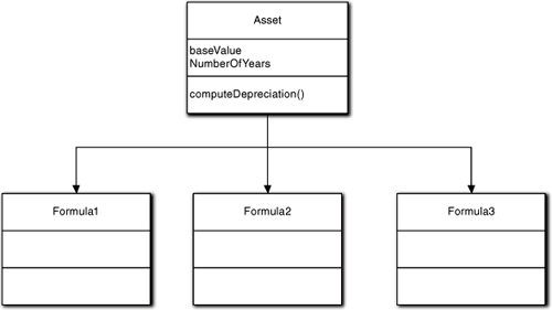
This replaces ad hoc polymorphism with the more elegant inclusion polymorphism. Instead of a single monolithic switch statement, we now isolate a specific formula to a subclass. This is the approach used by the Because It’s There School of OO Development; inclusion polymorphism is used because it is neat and uniquely OO rather than because the problem space requires it.

In many respects this solution is actually worse than the ad hoc polymorphism solution even though it looks more “OO-like.” That will become clear as soon as we need to subclass assets based on some other criteria (e.g., capital versus nondurable equipment). To accommodate the formula-based generalization, we will need a combinatorial number of subclasses that provide every possible combination of the two orthogonal classifications. A common variation on this solution is to use the Strategy design pattern, as shown in Figure 5-5.

Figure 5-5. Modeling depreciation using the Strategy pattern

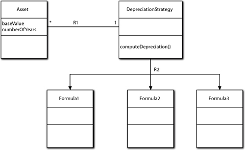
This eliminates any combinatorial subclassing because the depreciation algorithm has been removed from Asset entirely. However, it shares another problem with the previous example. If we want to add a new formula, we need to add a subclass. In addition, we need to modify the code that instantiates the R1 relationship. The only thing good about this solution is that it enables us to isolate and encapsulate the rules that determine which formula is the right one for the given Asset. In practice, that will usually involve the same sort of switch statement based on asset type as in the ad hoc polymorphic example, so we have just created some new objects that are close to being pure functions. Moral: Just because a neat feature exists in the OO paradigm does not mean one is required to use it.

To come up with a better solution that handles all the requirements in a quite elegant manner, we need to think about what the invariants of depreciation really are. In practice, the depreciation we compute is a single value that represents a fraction of the asset’s base value. That single value represents the amount to be amortized in a particular accounting period after the asset was acquired. That is, what we really need to compute is

We can compute the FractionInPeriod, for any formula for any year, t, after the asset acquisition without knowing anything about asset types as long as we know the total years of amortization. Thus for any year, t, all assets using the same formula for the same number of years of amortization will have exactly the same fraction of their base value for depreciation in that year.

The main insights here are (1) Computing the formula for a given amortization duration is always the same regardless of asset semantics and (2) Depreciation for a particular asset is nothing more than a fraction of its base value in any given accounting period. Both these insights represent useful invariants resulting from a decomposition of the problem until we were able to recognize essential elements. Why are these invariants useful? Consider Figure 5-6, which captures these insights.

Figure 5-6. Modeling depreciation invariants using a specification object

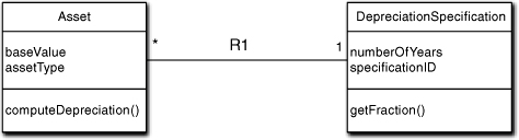
The answer lies in the fact that they allow us to employ parametric polymorphism to solve the problem in a very generic fashion. The “formula” that computeDepreciation now uses is the one above, which is exactly the same for any asset. We get the value of FractionInPeriod_t by navigating the R1 relationship and invoking getFraction with the desired value of t. All we have to do is supply it with the right value of baseValue for the asset. As in the inclusion polymorphism example, we get those by instantiating the R1 relationship correctly.

However, if we are clever about it, we can do that with a simple table lookup on assetType to yield the right specificationID. That mapping can be supplied in external configuration data rather then being encoded in executable statements. In addition, since DepreciationSpecification is just a dumb data holder, we can initialize all its instances from external configuration data as well. Then when an Asset object is created, we just do the lookup and instantiate the R1 relationship to the right instance in memory. The computeDepreciation behavior will then do the right thing for the asset.

Aside from a certain degree of elegance, the really neat thing is that we can add any number of new formulas and any arbitrary mapping between asset types and depreciation without touching the application model or the resulting implementation code. All we need to do is modify the external configuration data that defines DepreciationSpecification objects and the R1 relationship mapping between assetType and specificationID. That is, the actual computation of the formula is done once outside the application to supply the relevant values of FractionInPeriod_t for all combinations of formula and amortization duration in the definitions of DepreciationSpecification.

Now let’s take it one step further. The bean counters always have to provide you with three pieces of information whenever anything changes for depreciation: the formula to use, the asset type it applies to, and the amortization duration. You can create a data entry tool outside the application that the bean counters can use to provide that data. The tool provides a nice GUI with a couple of text boxes for asset type, amortization years, and specificationID along with a pick list for existing formulas to use. The tool then executes the formula and creates the configuration data without the bean counter knowing anything about trivia, like file formats.

If we really want to get exotic we can provide a UI that enables the bean counters to even provide new formulas off the cuff. (Think: the same sort of formula wizard as in a spreadsheet.) Now, it is hard to conceive of anything that could possibly change related to depreciation that would require an application modification. Better yet, the application is a whole lot simpler with a “formula” that has a single multiplication and assignment. You are probably not going to insert too many defects with that, especially when you don’t touch it in maintenance.

But haven’t we just moved the problem out of the application and into the tool the bean counters will use? Yes, we have, Grasshopper. Think of it as creating a distributed application where the elements communicate through the configuration file. However, we rack up some major gains in doing so—even if the total code lines in the tool are more than we would have had in any of the other computeDepreciation examples.

• Multiple contexts or even applications may need to compute depreciation. The infrastructure for reading and using the configuration data will be exactly the same for all of them.

• Depreciation will be computed far more often for assets than the formulas will be modified. We are simplifying what we do most often.

• Modifying a production application is nontrivial, and in most shops it can be a major undertaking. No production application needs to be modified here for most (if not all) possible changes to depreciation requirements. We have reduced the requirements changes to a data entry problem.

• The configuration data has a fixed format regardless of the requirements changes. All that changes are the values. Thus we only need to get the data entry application right once.

• Similarly, one only needs to get the processing of the configuration data right once, regardless of how many times the requirements change.

• The concerns are very well separated and decoupled. Formatting the configuration data from a very basic UI is a very narrowly focused problem for the data entry tool that has no distractions about the context of how the data will be used.

• The path from customer (bean counter) to the implementation for the requirements is very straightforward without a lot of opportunity for any misinterpretations, and such.

• When requirements do change, things like parallel testing of new configuration data are greatly facilitated because we just run the production application as usual. In fact, we could have the configuration data printed out in a format that would be easy for the bean counters to validate because they provided it as input in the first place.

In the end this approach to depreciation is an enormous win. It is curious that no one seems to do it this way. The big insight is simply that the depreciation in any time period is a fraction of the base value. When you read the new “formula” you knew exactly where we were going and probably thought to yourself, “Of course! Why didn’t I think of that?” The short answer is that most people don’t think of it because they are not used to thinking in terms of extracting invariants from the problem space.

Before leaving this example, note that it represents a special spin on the notion of invariant, compared to the last example. In the hardware register case the invariants were simply there for the picking; one just had to think about the problem space a bit more abstractly. In this case we needed to recast the problem space from a traditional view of computing depreciation to a different view of what the essential computation actually was. We did that by decomposing the elements of the process of computing depreciation until we could see a new pattern emerge. To do that we had to step back and think about how we used the value we computed. Thus the real invariant lay not in the computation itself but in the context of using its results.

Remote POS Entry Example

The next example is for a remote point-of-sale order entry system. For simplicity, we are concerned here only with the customer being able to create and submit an order for merchandise remotely from the vendor. We are going to ignore all other order processing at the vendor once the order is received. In this case, let’s assume there is a general merchandiser with a wide variety of items for sale in many different goods categories.

Let’s further assume that some cross-functional team went out and beat the bushes with real customers to come up with the following set of requirements. (Though the list has the correct level of ambiguity, it is shorter than one in real life would be; this is just a representative example to make a point.)

• The goods need to be categorized in a hierarchy (e.g., clothing → men’s → sportswear). The categories will follow the existing standard inventory classification system.

• The customer needs a convenient mechanism to navigate the goods categories.

• Major goods categories need to be immediately accessible from anywhere in the order entry process except order submission processing.

• A search facility must be provided to find all categories of goods or specific items.

• The customer can order one or more items. A list of currently desired items will be maintained. The customer needs to be able to easily review the list and add or remove items from it. The items in the list are not actually ordered until the customer submits the order.

• Customers need to be able to review every aspect of the order, including total cost adjusted for shipping fees, discounts, and taxes.

• Goods descriptions must be displayed in a consistent format. Required order attributes (size, color, style, etc.) must be separated from other descriptive material and emphasized.

As you read the list of requirements did you think: Web, Hyperlink, and Shopping Cart?

Bzzzzzt! Thanks for playing. You have just flunked your first pop quiz on modeling invariants.

About a century ago Sears solved this problem by placing a mail order catalogue in a large fraction of the homes in the United States. That catalogue had solutions for every one of the listed requirements. For example, it had color-coded pages and an index for easily finding categories of items and individual items; it had an order form to record desired goods, and the customer could add or remove items from the form; and submission was clearly defined by mailing the order form back to Sears. The fundamentals of remote POS order entry have not changed in that time. The only things, aside from prices, that have changed are the implementation mechanisms.

Note that most general merchandisers still have mail order catalogues alongside their spiffy new web sites. This fact should be suggestive. It would be highly desirable to use the same software infrastructure for both mail order and web orders. For example, the order descriptions should be displayed the same way on the web and in the catalogue to allow reuse in the web display software and the print layout software. For consistency, all the item description information should be in one place. The same categorization, in fact, must be used because that is a standard referenced in the requirements. Also, the software that processes the orders would like to be indifferent about where the order originated.

The assertion here is that the OOA model should look exactly the same for the modern web implementation and the century-old Sears manual solution. One very good yardstick used by reviewers to ensure that OOA models are implementation-independent is that the model could be implemented as a manual system, like the Sears mail-order catalogue, in the customer’s environment without changing the model. Essentially, this means that the OOA model must be sufficiently abstract to describe both a manual and a computerized solution.

We are not going to go through a detailed OOA model here to demonstrate invariants for this example. That is mostly a matter of class-level abstraction, and we will be dealing with that a lot more Part II. Instead, it will be left as a class exercise to think about how one would describe a solution abstractly enough that it would be accurate for such disparate solutions as web and mail order implementations.

Here is one hint of things to come, though. In the requirements, the notion of categories of goods was quite dominant. It would be very tempting to create a taxonomy of goods where every item type (class) was a leaf subtype in a monolithic generalization structure. After all, generalization is one of the distinctive characteristics of OT, right? And groups of items will share characteristics like size that can be captured in superclasses, right? For reasons we will get to later, that would be a serious error because it would invite major problems in doing maintenance as new categories and items were added and removed in the future.

For now just note that categories exist in the requirements for one and only one reason: to make navigation through the items easier for the customer. That context has nothing to do with the inherent characteristics of goods. Superficially there is a sharing of characteristics. For example, women’s shoes and men’s coats have a size, while refrigerators and air conditioners have an energy rating. But if you try to organize shared characteristics into a monolithic inheritance hierarchy for anything as complex and volatile as a general merchandiser’s inventory, you will have nightmares about overweight duck-billed platypuses chasing you through mazes.

Once we recognize the role of categories as a navigational aid, we can focus on the invariants of navigation. Separation of a navigation representation from item representation can result in an elegant simplification where the entire navigational hierarchy is represented with only two classes, as shown in Figure 5-7. The object relationships that are represented by the reflexive parent/child relationship on Category contain all of the hierarchical information in a form that is ideally suited for navigating to the immediately higher or lower levels around a given category.

Figure 5-7. Example of using a reflexive relationship to describe a tree hierarchy

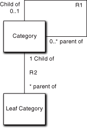
Figure 5-7 is a classic model of a hierarchical tree. The structure of the navigation is completely captured in the relationships. We can write the software for any hierarchical navigation (e.g., “walking” a web site like Amazon.com) from this model. The reason that Leaf Category is special is because we need to actually display inventory items when the user gets to that level. But we can accommodate even that in a generic fashion in Figure 5-8.

Figure 5-8. Separation of the invariants for hierarchy navigation and hierarchy content

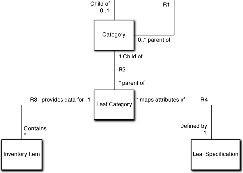
In this representation the Leaf Category class represents a collection of real items in the lowest leaf-level category. We can extend this by providing a Leaf Specification class that defines the attributes that are relevant for all the items in the leaf category. The Leaf Specification tells the Leaf Category how to interpret the data in the relevant Inventory Items. Essentially, this maps generic items’ attribute values into characteristic semantics that will be relevant to the customer (e.g., the item’s third attribute value, say 8 in an item instance, will always map into a women’s dress size in the display).

The details of how to do this are a bit tricky so we will defer them until we get to class-level modeling. The important thing to note here, though, is that all the instances of Category, Leaf Category, and Leaf Specification and their relationships can be created at runtime from external data. This enables us to arbitrarily add or remove categories and item types without touching the software; it can all be done in the external data. Thus this marvelously simple model solves the entire navigation problem and enables virtually any type of new merchandise to be added to the inventory without changing the model.

Also note that we have specified the hierarchical POS category navigation but not the organization of Inventory Items. The requirements indicated they needed to be the same and that is fine. But the organization of Inventory Items doesn’t really matter to the POS navigation problem, so we don’t say how we know which Inventory Items go with a particular Leaf Category. All we need is a list of Inventory Items that goes with a Leaf Category, and that also can be defined in an external configuration file.⁹

We got to this model by stepping back and focusing upon the navigation problem invariants without worrying about the nature of specific goods. In doing that we recognized that navigation was about “walking” a hierarchical tree structure rather than generalization. That is, the relevant invariant is that navigation is about parent/ child relationships between entities, not the inherent characteristics of the entities themselves. From there, modeling the tree structure alone was relatively easy.

Another key insight was that we don’t care about how actual Inventory Items are organized. The requirements say that the categories will have to map the same way, but we do that outside the application where the configuration data is defined. That is, the rules for construction of the configuration data that defines R1 will be driven by the organization of Inventory Items. This is important to long-term robustness for two reasons. It means that requirements can change without affecting our POS software. Perhaps more important, it means we can focus on a much narrower problem in the POS without worrying about merging two different structures. That leads to an elegantly simple solution without any other concerns that drive why the Inventory Items are organized in a particular way. That simplicity would be impossible without having first decided that a POS was a different subject matter from Inventory Control that had different invariant concerns.