2.3. Toxic Effects
One of the major hazards that could be present in a facility is the release of a toxic chemical. In general, this type of hazard depends on various different elements such as the conditions of exposure and on the properties of the substance that is being released. To determine the effects, one should focus on both: brief exposures at high concentrations and prolonged exposures at low concentrations. For instance, release of a very toxic chemical such as chlorine should be treated with caution as it could disperse through large areas and have much larger effect than those of fires or explosions leading to catastrophic incidents. Although the toxic releases occur less frequently than a fire or explosion still, the scenario should always be considered of high importance.
The First Report of the Advisory Committee on Major Hazards (ACMH) states (Harvey, 1976):
“With toxic materials, the sudden release of very large quantities could conceivably cause even larger numbers of casualties than a flammable escape. In theory such a release could, in certain weather conditions, produce lethal concentrations in places 20 miles from the point of release but the actual number of casualties (if any) would depend on the population density in the path of the cloud and the effectiveness of the emergency arrangements that might include evacuation.”
As stated, dispersion of toxic substances can travel long distances and, consequently, the long-term toxic effects due to the exposure at low concentrations of certain chemicals can affect a large part of the population.
This section covers the different routes of how toxic substances can enter an organism. A clear distinction between these mechanisms is established. Then a brief overview of toxic substances and how these can be identified in Material Safety Data Sheets (MSDSs) are shown. Subsequently, a description of a toxic assessment is given. In this part, it is briefly described how Environmental Protection Agency (EPA) establishes a distinction between cancer and noncancer effects. Additionally, in this section, the effects of toxic substances, limit values set for these in the United States of America are shown and the different approaches employed by federal agencies such as the Occupational Safety and Health Administration (OSHA) and the EPA to regulate these chemicals is presented along with the assessment of the hazards of toxic releases. It should be kept in mind that this chapter presents an engineering approach on how to avoid toxic releases and illustrates how the federal agencies work together to establish and implement regulations and how should these regulations should be interpreted for assessments of short- and long-term effects.
2.3.1. How Toxic Substances Enter the Organism
In general, toxic substances can enter biological organisms via any of the following routes:
• Dermal absorption
• Injection
• Inhalation
• Ingestion
For every possible route, there is a method of control. For instance, ingestion can be controlled by reinforcement of rules on eating, drinking, and smoking; inhalation can be controlled by ventilation, respirators, and personal protection equipment; and injection and dermal absorption by proper protective clothing. Moreover, the smaller the particle size, the more probable it is for the particle to translocate from any of the entry routes into the circulatory and lymphatic systems following to the organs and tissues. Some particles, depending on their size and composition, may produce irreversible damages to cells or organelle injury. Figure 2.14 shows an example of a cell compared with different sizes of particles.
2.3.2. Particle Classification
Particles can be classified based on dimensionality, morphology, composition, uniformity, and agglomeration. In general, motion of particles is not limited, and they can interact with humans with no difficulty; however, the smaller the particle is, the greater the health hazard is. At this point, it is important to clarify that not all particles are toxic, as toxicity is a function of chemical composition and shape. Additionally, classification of toxicity is limited and further research should be addressed for each material and morphology. In the following sections, a typical classification of the particles is given.

Figure 2.14 Size comparison between cells and other particles (Buzea et al., 2007).
2.3.2.1. Dimensionality
A number of dimensions are used to classify particles. In other words, this is a generalization of the “aspect ratio” concept (Buzea et al., 2007). There are three different categories; one-dimensional (1D), two-dimensional (2D), and 3D materials.
• 1D materials: In the nanometer scale, these are thin films or surface coatings. An example of 1D materials is carbon nanotubes.
• 2D materials: These types of materials have two dimensions in the nanometer scale. An example of 2D materials is asbestos fibers.
• 3D materials: These types of materials have three dimensions in the nanometer scale. Examples of 3D materials are colloids and nanoparticles.
2.3.2.2. Particle morphology
The morphology plays an important role when classifying a particle. For instance, flatness, sphericity, and aspect ratio are the more important characteristics to be taken into account.
2.3.2.3. Particle composition
In general, particles can be composed of a single material or a composite of several materials (Buzea et al., 2007).
2.3.2.4. Particle uniformity and agglomeration
Particles can exist as dispersed aerosols, suspensions/colloids, or in an agglomerated state. In the agglomerate state, particles may behave as larger particles, and their behavior will depend on the size of the agglomerate.
2.3.3. Toxic Substances
In essence, all chemical substances can cause adverse health effects if the chemical is induced in high doses; however, when the dose is low, typically no health effect is observed. There are some factors that should be kept in mind when dealing with toxic substances. Most of them can be found in the MSDS of the chemical substance and the following is a list of some of the factors (Mannan, 2012):
1. Generation of the substance
2. Toxic concentrations
3. Effects of exposure
4. Detectability by odor
5. Precautions in handling
6. Leak detection
7. First aid
Chemicals evolve along with technology and the use or production of toxic chemicals. Several of the toxic substances that present hazards for people and the environment are produced, and some of them are generated as byproducts of the process. For instance, carbon monoxide, produced by an incomplete combustion process, is an asphyxiant gas. In general, to achieve complete combustion is very difficult as there are many reactions that can be involved during the progress of the reaction. Another example is nitrogen oxides, which can be produced during welding processes. Nitrogen oxides present an irritant effect but on inhalation could be fatal.
As mentioned, chemicals evolve along with technology, and every year the number of chemicals produced increases. Studies performed by Langley (1978) identified that in the decade prior to 1978, a total of 4 million new chemicals were identified. From such a large quantity, it was estimated that the United Kingdom had 300–400 new chemicals per year, and the United States tends to duplicate such values.
Some of the problems related to exposure of toxic chemicals vary based on the time of exposure. For instance, noxious effects can result from continuous exposure to a substance that presents a level of toxicity that has not been appreciated. However, some toxic chemicals may cause cancer and malfunction of different human organs. In the following paragraphs, a more detailed explanation about different hazardous particles is given.
The human body needs several metals for proper functioning. However, it has been proved (Shah, 1998) that exposure to high levels of these metals can have an adverse health effect. In general, the smaller the particle, the higher are the chances for it to get into the organism. Therefore, activities such as dealing with or manufacturing nano- and micro-sized particles should be considered as a serious occupational hazard. In general, the inhalation of dusts is well known to have an adverse health effect. Moreover, the health effect they can cause is a function of the material itself, the exposure duration, and the dose. For instance, exposure to metal dust, such as platinum, nickel, or cobalt, can cause asthma, while the inhalation of other metallic dusts can lead to pulmonary fibrosis and lung cancer. In the following paragraphs, some examples of dusts and the effect of being exposed to them are discussed.
Lead: When lead is inhaled or ingested, it circulates in the blood and gets deposited in bone and other tissue. Chronic exposure to lead can cause impairment of mental functions, visuomotor performance, attention span, anemia, and kidney disease, among others (Shah, 1998).
Cadmium: High-dose exposure to cadmium leads to lung irritation, nausea, and vomiting. Long-term and low-dosage exposure in humans can cause lung emphysema and central and nervous system and liver damage. Lung cancer has also been related to exposure to cadmium. It is important to mention that cadmium is present in industrial and consumer waste, which leads to accumulation of cadmium in soil. Consequently, plants and crops are growing in a contaminated soil, leading to a contamination of vegetables and animals (Shah, 1998).
Iron: Even though small doses of iron are essential to ensure survival, it has been proven experimentally that high-dose exposure to iron in animals can lead to an increased risk of developing cancer. In humans, high-dose exposure to iron has been linked to cause sarcomas at the sites of deposition, liver cancer, and neurological diseases, such as Parkinson‘s and Alzheimer‘s diseases.
Beryllium: Inhalation of beryllium can lead to lung damage, hypersensitivity, and beryllium disease. Long-term exposure can increase risk of lung cancer in humans (Paris et al., 2004).
Aluminum: Long-term exposure to aluminum leads to anemia, bone disease, dementia, and breast cancer diagnosis (McGrath, 2003). Further, studies have proven that the brain plaque of people with Alzheimer‘s disease has high levels of aluminum (Shah, 1998).
2.3.4. Toxicity Assessment
Toxicity assessment is used to identify the potential adverse health effects that a chemical can cause and determine how the appearance of these effects depends on the exposure level (dose). As mentioned, the toxic effects of a chemical depends on the route, dosage, and duration of exposure. Therefore, toxic chemicals must have a list of potential adverse effects and the frequency of such effects is noted based on the dose, route, and duration of exposure. According to the EPA (1991), the toxicity assessment process is divided into two parts. The first part characterizes and quantifies the noncancer effects of the chemical. The second part addresses the cancer effects of the chemical.
As mentioned earlier in this section, all chemicals can cause adverse health effects. However, for this to occur, exposure to the chemicals has to occur at a sufficiently high dose. If the dose is not sufficiently high, depending of the chemical, normally there is no adverse health effects. Therefore, for toxic substances, it is important to establish a threshold dose at which adverse effects become evident. As mentioned, not all particles produce adverse health effects; the toxicity depends on various factors, such as size, composition, crystallinity, and aggregation, among others. Moreover, the toxicity of particles to organisms depends on the organism genetic complement, which provides either ways to adapt or fight toxic substances. It has been found that the inhalation of certain nanoparticles is associated with certain diseases such as asthma, lung cancer, and Parkinson‘s and Alzheimer‘s diseases. Further, research has proved the presence of nanoparticles in the circulatory system in several cases of heart disease, arrhythmia, or arteriosclerosis.
2.3.4.1. Noncancer effect
In general, the threshold dose is established from toxicological data. These data come from studies on humans and/or animals and consists of determining the highest dose that does not cause any observable adverse effect, called no observed adverse effect level (NOAEL), and the lowest dose that produces an effect, called the lowest observed adverse effect level (LOAEL). As there is an interval between the LOAEL and the NOAEL, a threshold should lie in between these values (EPA, 1991).
To determine a threshold value, a reference dose (Rd.) is estimated from the NOAEL. If there is no NOAEL reported, then the Rd. value is derived from the LOAEL. In any case, the NOAEL or LOAEL is divided by an uncertainty factor. In cases when the data are sufficiently reliable the uncertainty factor can be as small as 1. However, when there are limited data, the uncertainty factor can be as high as 10. In general, the Rd. is an estimate of a daily exposure of the human population that is likely to be affected by the hazardous effects of a chemical substance during a lifetime (Allport et al., 2003).
2.3.4.2. Cancer effect
In this case, toxicity assessment process has two components. The first is a qualitative evaluation of the weight of evidence that the chemical can or cannot cause cancer in humans. The second part of this assessment is only for chemicals that are believed to be capable of causing cancer in humans; in other words, the main goal is to describe the carcinogenic potency of a chemical. This is done by quantifying how the number of cancers on humans and/or animals increases as the dose increases (EPA, 1991).
2.3.5. Risk Assessment
In general, the information that can be obtained from toxicity assessments could be used to assess the toxic risk of a facility. However, as shown before, there are two different approaches to assess the risk due to toxic chemicals. The first one is proposed by federal agencies in the form of regulations. These regulations help to limit all the different companies that are covered by them. The other approach is the one carried out by the manufacturer for facility design and operation purposes.
There are several other methodologies for risk assessment in the federal government. Some of them are managing the process (NAS/NRC, 1983), assessment and management of chemical risks (Rodricks and Tardiff, 1984), toxicological risk assessment (Clayson et al., 1985), and the risk assessment of environmental hazards (Paustenbach, 1989; Bridges, 1985; Nabholz, 1991; Becking, 1995; Frederick, 1995; Mannan, 2012).
Furthermore, according to the National Academy of Sciences (NAS) report, risk assessment consists of four different stages (National Research Council, 1983; Cohrssen and Covello, 1999):
• Hazard identification: At this stage, a list of chemicals that can have an adverse effect is made. Additionally, a list of possible health problems that can arise due to exposure is considered. Here, several factors are accounted, such as the type and severity of the effects, route of exposure, and frequency of exposure.
• Dose–response assessment: Determine how a specific chemical can affect adversely human being's health at different doses.
• Exposure assessment: Determine the working capabilities of a facility. Questions addressed are, for example, How many hours is a worker exposed to a toxic substance? How many people are exposed during a certain period of time?
• Risk characterization: In this stage, the extra risk of health problems in the population that has been exposed to the chemical is analyzed.
At this point, various issues regarding toxic chemicals have been addressed. For instance, dose–response and TRA have been studied briefly. It is clear that there is a need for establishing thresholds to avoid adverse health effects. Still, the level of exposure to be expected has to be defined. This is performed by using the suitable risk criteria.
Toxic risk assessment has been used to define hygiene standards, especially in the United States. For example, for inorganic arsenic, OSHA used a linear dose–response model. In such a case, OSHA has stated that for every 1000 workers over a working lifetime, there could be a maximum of eight deaths at a level of 10 mg/m3, 40 at 50 mg/m3, and 400 at 500 mg/m3. On the basis of this standard, the dose was reduced from 500 to 10 mg/m3. To justify this decision, OSHA stated (Mannan, 2012):
“The level of risk from working a lifetime of exposure at 10 mg/m3 is estimated at approximately 8 excess lung cancer deaths per 1000 employees. OSHA believes that this level of risk does not appear to be insignificant. It is below risk levels in high-risk occupations but it is above risk levels in occupations with average levels of risk.”
2.3.6. Hygiene Standards
As discussed before in the beginning of this chapter, there are two different types of toxic exposures: brief exposures at high concentrations and prolonged exposures at low concentrations. In general, the American Conference of Governmental Industrial Hygienists (ACGIH) establishes thresholds for different toxic substances. For instance, these thresholds are determined to avoid intoxication and, therefore, permit the body to detoxify and eliminate the toxic substance without showing any adverse health effect.
Threshold limit values (TLVs) refer to airborne concentrations that correspond to conditions under which no adverse health effect is expected during a worker's lifetime. It is assumed that the exposure is going to occur 8 h per day and 5 days per week (Crowl and Louvar, 2011).
There are three different types of TLVs. They are described in Table 2.3:
Table 2.3
Definitions for Threshold Limit Values (TLVs) (Crowl and Louvar, 2011)
| TLV Type | Definition |
| TLV-TWA | TLV time-weighted average |
| The concentration for a conventional 8-h workday and a 40-h work week, to which it is believed that nearly all workers may be repeatedly exposed, day after day, for a working lifetime without adverse effect. | |
| TLV-STEL | TLV short-term exposure limit |
| A 15-min TWA exposure that should not be exceeded at any time during a workday, even if the 8-h TWA is within the TLV-TWA. The TLV-STEL is the concentration to which it is believed that workers can be exposed continuously for a short period of time without suffering (1) irritation, (2) chronic or irreversible tissue damage, (3) dose rate–dependent toxic effects, or (4) narcosis of sufficient degree to increase the likelihood of accidental injury, impaired self-rescue, or materially reduced work efficiency. Exposures above the TLV-TWA up to the TLV-STEL should be less than 15 min and should occur no more than four times per day, and there should be at least 60 min between successive exposures in this range. | |
| TLV-C | TLV ceiling |
| The concentration should not be exceeded during any part of the working exposure. |

Table 2.3 describes exposure under working conditions, but exposures under emergency conditions are determined using probit equations. However, this approach is very limited, because data are available and published for a limited amount of chemicals. A secondary approach is to specify a toxic concentration criterion above which the interaction with the toxic substance can have adverse health effects. Some of these methods and criteria are described next (Crowl and Louvar, 2011):
• Emergency response planning guidelines (ERPGs) for air contaminants by AIHA
• Immediately dangerous to life or health (IDLH) levels by NIOSH
• Emergency exposure guidance levels (EEGLs) and short-term public emergency guideline levels (SPEGLs) by NAS/NRC
• Permissible exposure limits (PELs) by OSHA
• Toxicity dispersion (TXDS) by New Jersey Department of Environmental Protection
• Toxic end points by EPA
2.3.6.1. ERPG
The concentration ranges given by the ERPGs are provided as a consequence of exposure to a specific substance. There are three different levels for ERPGs.
ERPG-1 is the maximum airborne concentration below which a person could be exposed for 1 h and there is a transient adverse health effect or perceiving an objectionable odor.
ERPG-2 is the maximum airborne concentration below which a person could be exposed for up to 1 h without having an irreversible or a serious adverse health effect that could avoid the person to take any protective action.
ERPG-3 is the maximum airborne concentration below which all the population could be exposed for up to 1 h without developing life-threatening health effects.
2.3.6.2. IDLH
This criterion allows the identification of acute toxicity doses for certain industrial gases. NIOSH defines IDLH as “that poses a threat of exposure to airborne contaminants when that exposure is likely to cause death or immediate or delayed permanent adverse health effects or prevent escape from such an environment” (NIOSH, 2005). It is important to mention that the IDLH level is considered a maximum concentration above which only a breathing apparatus, such as a self-contained breathing apparatus (SCBA), is permitted. If these values are exceeded, all workers who do not have protection must leave the area immediately.
2.3.6.3. EEGL
EEGL is the concentration of a gas, vapor, or aerosol that is acceptable and allows exposure to perform specific tasks during emergency conditions that last between 1 and 24 h. In general, when a person is exposed to an EEGL concentration, possible effects such as irritation of the central nervous system that do not produce long-term adverse health effects or that would impair performance of a task.
SPEGL is the acceptable concentration for exposures of the general public. In general, SPEGL values are set between 10% and 50% of the EEGL and takes into account different types of population (i.e., the elderly, children, infants).
2.3.6.4. PEL
PEL values are comparable to the TLV values as they take into account a time-weighted average exposure of 8 h. In fact, the main difference between the PELs and the TLVs is the agency from which they come. PELs are developed and published by OSHA.
2.3.6.5. TXDS
New Jersey uses a consequence analysis methodology to estimate the catastrophic quantities of toxic substances. This is required by the New Jersey Toxic Catastrophe Prevention Act (TCPA). In general, acute toxic concentrations are defined as the exposed concentration at which a toxic substance can cause acute health effects in the affected population and one fatality of 20 or fewer during a 1-h exposure.
2.3.6.6. RMP
In general, EPA's RMP requires that if a facility is handling a toxic substance that is listed as an extremely hazardous substance, dispersion modeling should be performed. This list of substances can be found in the document titled Consolidated List of Chemicals Subject to the Emergency Planning and Community Right-To-Know Act (EPCRA), Comprehensive Environmental Response, Compensation and Liability Act (CERCLA) and Section 112(r) of the Clean Air Act. In this study, a toxic end point must be used as a reference. EPA has an order of preference for these simulation scenarios. The first one is the ERPG-2 and the second one is the level of concern, which can be found in the EPCRA. According to the EPA, the level of concern is “the maximum concentration of an extremely hazardous substance in air that will not cause serious irreversible health effects in the general population when exposed to the substance for relative short duration” (EPA, 1996).
2.3.7. Hazard Assessment Methodology
Before heading deeper into hazard analysis, it is important to clarify what is a hazard. According to OSHA, “a hazard is the potential for harm. In practical terms, a hazard often is associated with a condition or activity that, if left uncontrolled, can result in an injury or illness” (OSHA, 2002).
To perform a hazard analysis is usually very challenging. The level of complexity for this type of analysis is subject to the level of detail the hazard analysis team wants to go into. For instance, if there are potential hazards that could affect a nearby population, such detail is essential. On the other hand, it is possible to disregard a scenario that will not cause any harm to any person. For example, the team is evaluating many processes and operations, but they realize that from 10 operations, only three have the potential to harm people. It may be sufficient to analyze those three scenarios, because the other seven scenarios do not have a chance to affect the nearby population. There are several types of hazard analysis. All of them are different and present a different procedure of how to assemble a team and how to analyze such hazards.
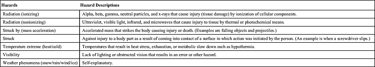
According to OSHA, one of the easiest and possibly most effective methods is the job hazard analysis (JHA), also known as job safety analysis (JSA). In general, a JHA focuses on job tasks as a way to identify hazards before they occur. At the same time, it finds a relationship between the worker, the tasks, the tools, and the work environment. The main purposes of the JSA are to identify hazards that are not controlled and to take appropriate measures to either prevent the hazard or reduce it to an acceptable risk level. Table 2.4, identifies the major type of hazards that can be identified on a JHA (OSHA, 2002).
Table 2.4
Hazards Identified by a JHA (OSHA, 2002)
| Hazards | Hazard Descriptions |
| Chemical (toxic) | A chemical that exposes a person by absorption through the skin, inhalation, or through the bloodstream that causes illness, disease, or death. The amount of chemical exposure is critical in determining hazardous effects. Check material safety data sheets (MSDSs) and/or OSHA 1910.1000 for chemical hazard information. |
| Chemical (flammable) | A chemical that, when exposed to a heat ignition source, results in combustion. Typically, the lower a chemical's flash point and boiling point, the more flammable is the chemical. Check MSDS for flammability information. |
| Chemical (corrosive) | A chemical that, when it comes into contact with (corrosive) skin, metal, or other materials, damages the materials. Acids and bases are examples of corrosives. |
| Explosion (chemical reaction) | Self-explanatory. |
| Explosion (over pressurization) | Sudden and violent release of a large amount of gas/energy due to a significant pressure difference such as rupture in a boiler or compressed gas cylinder. |
| Electrical (shock/short circuit) | Contact with exposed conductors or a device that is incorrectly or inadvertently grounded, such as when a metal ladder comes into contact with power lines. A 60-Hz alternating current (common house current) is very dangerous because it can stop the heart. |
| Electrical (fire) | Use of electrical power that results in electrical overheating or arcing to the point of combustion or ignition of flammables, or electrical component damage. |
| Electrical (static/ESD) | The moving or rubbing of wool, nylon, other synthetic fibers, and even flowing liquids can generate static electricity. This creates an excess or deficiency of electrons on the surface of material that discharges (spark) to the ground resulting in the ignition of flammables or damage to electronics or the body's nervous system. |
| Electrical (loss of power) | Safety-critical equipment failure as a result of loss of power. |
| Ergonomics (strain) | Damage of tissue due to overexertion (strains and sprains) or repetitive motion. |
| Ergonomics (human error) | A system design, procedure, or equipment that is error provocative. (A switch goes up to turn something off.) |
| Excavation (collapse) | Soil collapse in a trench or excavation as a result of improper or inadequate shoring. Soil type is critical in determining the hazard likelihood. |
| Fall (impacts) | Conditions that result in falls from (slip, trip) height or traditional walking surfaces (such as slippery floors, poor housekeeping, uneven walking surfaces, exposed ledges). |
| Fire/heat | Temperatures that can cause burns to the skin or damage to other organs. Fires require a heat source, fuel, and oxygen. |
| Mechanical/vibration (chaffing/fatigue) | Vibration that can cause damage to nerve endings, or material fatigue that results in a safety-critical failure. (Examples are abraded slings and ropes, weakened hoses and belts.) |
| Mechanical failure | Self-explanatory; typically occurs when devices exceed designed capacity or are inadequately maintained. |
| Mechanical | Skin, muscle, or body part exposed to crushing, caught-between, cutting, tearing, shearing items or equipment. |
| Noise | Noise levels (>85 dBA 8-h TWA) that result in hearing damage or inability to communicate safety-critical information. |
| Table Continued | |

| Hazards | Hazard Descriptions |
| Radiation (ionizing) | Alpha, beta, gamma, neutral particles, and x-rays that cause injury (tissue damage) by ionization of cellular components. |
| Radiation (nonionizing) | Ultraviolet, visible light, infrared, and microwaves that cause injury to tissue by thermal or photochemical means. |
| Struck by (mass acceleration) | Accelerated mass that strikes the body causing injury or death. (Examples are falling objects and projectiles.) |
| Struck | Against injury to a body part as a result of coming into contact of a surface in which action was initiated by the person. (An example is when a screwdriver slips.) |
| Temperature extreme (heat/cold) | Temperatures that result in heat stress, exhaustion, or metabolic slow down such as hypothermia. |
| Visibility | Lack of lighting or obstructed vision that results in an error or other hazard. |
| Weather phenomena (snow/rain/wind/ice) | Self-explanatory. |
2.3.8. Source Term
When dispersion of a substance occurs, two stages can be identified. The first is the source term, and the second one is atmospheric dispersion. In general, the source term occurs right after the release, when the behavior of the fluid is dominated by the storage conditions and the conditions of release. After the influence of the source starts decaying, the atmospheric dispersion starts ruling over the source term. Figure 2.15 illustrates the possible emissions situations.
There are two different types of releases. The first one is the continuous release, and the second one is the instantaneous release. In general, there is a criterion to determine what type of release is occurring. A continuous release is defined by the following relation:
![]() (2.86)
(2.86)
where ux is the friction velocity. According to Mannan (2012), Eqn (2.86) implies that at a certain distance x where the release can be regarded as continuous recedes closer to the source as the duration of the release decreases to T0. If distances are much greater than the ones given by Eqn (2.86), there will be an overestimate in the concentration. Now, to determine if the release is instantaneous, the following relation must be applied:
![]() (2.87)
(2.87)
It can be noticed that there is a gap between continuous and instantaneous release. In this gap, the release behaves neither as continuous nor as instantaneous; it is a transient release. The release thus can be described as quasi-continuous or quasi-instantaneous. In general, quasi-continuous release can be treated as follows: the total amount of substance released Q0 over the duration of the release T0 gives an effective release rate q0. With this release rate, it is possible to obtain the concentration at a certain distance. If the release is treated as an instantaneous release, the only parameter that has to be used is the total amount of substance released Q0 (Mannan, 2012).

Figure 2.15 Some emissions situations (Mannan, 2012).
2.3.9. Gas Dispersion
In most cases, the vapors of the principal toxic liquids exhibit heavy gas behavior and great strides have been made in heavy gas dispersion modeling. It is important to mention that there are four categories in which most of the models can be found. These classes are:
• Workbooks/correlations
• Integral models
• Shallow layer models
• Computational fluid dynamics (CFD) models
Most of the commercial or publicly available models belong to one of these categories and can be found in Table 2.9 (Luketa-Hanlin, 2006).
2.3.9.1. Workbooks/correlations
These types of models are recognized, especially due to the simplicity of their calculations (compared with different groups). There are many models of this type that can predict the concentration profile of gases that are being dispersed downstream. These types of models have been validated against experimental data, such as Britter and McQuaid's and the Gaussian Plume Model (GPM) (Luketa-Hanlin, 2006).
2.3.9.2. Integral models
These types of models are much more complex than workbook/correlation models. They include the solutions of basic differential equations. However, it is important to note that most of these types of models tend to idealize atmospheric conditions and some terrain descriptions (they assume that the terrain is plain and the dispersion is not going to be affected by any obstruction), and some of these models do not allow for the inclusion of geometry, making it difficult to simulate different obstacles and allowing for uncertainty in the calculations. When a complex scenario (with obstacles) is going to be simulated, most of the results obtained in this type of simulation will not be entirely trustworthy (Luketa-Hanlin, 2006). Many models of this kind have been successfully validated against experimental data.
2.3.9.3. Shallow layer models
This group has characteristics of the CFD models and the integral models. For example, some models will allow the inclusion of geometry in the simulation. The properties such as temperature, concentration and cloud height are modeled on horizontal coordinates in a depth integral sense. Basically, most of these types of models are used as research tools (Luketa-Hanlin, 2006).
2.3.9.4. Computational fluid dynamics
This group uses the Navier–Stokes equations to predict how the dispersion of a gas is going to behave and presents the results in three dimensions. These models allow for the inclusion of geometry and correctly specify the scenario. However, these models are highly sensitive to the scenario setup. The user has to be extremely aware and have a wide understanding of this peculiarity. The major problems with CFD models include their large use of computer resources and time and their need for a person who has expertise in the CFD simulation field (Webber et al., 2010; Britter and McQuaid, 1988; Cormier, 2008; Hansen et al., 2010).
Appropriate use of these models allows the replication of experiments that are performed in wind tunnels. Furthermore, wind tunnel experiments allow to include obstruction in a terrain and to study the effect of slopes, buildings, barriers, and water spray curtains. In general, the concentrations obtained by these models (mostly used for heavy gas dispersion) are very different to the results obtained in passive gas dispersion models (such as the Gaussian Model).
2.3.10. Concentration Fluctuations
In general, most models predict a concentration average. Such average is the most expected concentration for the prescribed input conditions at certain point. For example, if various experiments are performed identically (with the same atmospheric and release conditions), this average would represent the average of the amount of experiments performed. In reality, this is extremely difficult to perform as there is always turbulence in the environment. Therefore, if the same experiment is performed twice, it is very likely to obtain two different concentration averages in the same place. This is what dispersion models do. They do not show the concentration fluctuation around a point; they average the concentration fluctuation in that point and the response that is given is the simple average of these fluctuations (CCPS, 1996).
From this, it has been shown that at a fixed point the concentration fluctuates considerably in a vapor cloud. Griffiths and Harper (1985) mentioned that these concentration fluctuations have influence on the effective toxic load (Wilson and Simms, 1985; Wilson, 1991; Blewitt et al., 1987; Davies, 1987, 1989) and propose some methods to treat this influence.
2.3.11. Mitigation: Terrain, Barriers, Sprays, Shelter, and Evacuation
When a dispersion event occurs in a facility, there are several parameters that can affect the behavior of the dispersion. For instance, if a heavy gas is being dispersed; such gas will tend to be near the ground. Particular attention should be given to these types of scenarios, as these types of releases tend to affect large areas (Busini et al., 2012). In this specific case, the terrain will play an important role. For example, if there is a sharp slope upwards it will be more difficult for the gas to disperse. On the contrary, if there is a sharp slope downward, the gas will disperse with ease. An important parameter to take into account when studying this type of scenarios is the surface roughness. The surface roughness will create certain friction between the gas cloud and the floor. This force will slow down the velocity of dispersion and, consequently, the size of the flammable cloud. This situation can be observed when there is a high surface roughness (TNO, 2005).
There are different methods to mitigate dispersion and reduce the size of the toxic cloud. For instance, the inclusion of barriers in the system may diminish the size of the cloud. In general, barriers are installed near the location of a possible leak. The purpose of the barriers is to contain as much gas as possible and make it more difficult for the gas to go around it and keep dispersing. Several types of barriers are used; some substances are regulated to be stored in vessels and those vessels, at the same time, must be in dikes.
From the discussion regarding the different types of models, it is clear that the only model capable of predicting how a gas is going to be dispersed in presence of obstacles, like in a facility, is the CFD model (Mannan, 2012). Therefore, when simulations are going to be performed for a certain facility, it is preferable to use CFD models. However, as CFD models demand a great amount of time, a balance between precision and estimate should be made. In other words, using CFD models for simple geometries can be a waste of time, and this type of scenarios could be studied using integral models. Figure 2.16 illustrates how different outcomes are obtained when there are obstacles included in the scenario and when the scenario does not have any obstruction.
As can be observed in Figure 2.16, the obstacles present in the scenario significantly reduce the downwind distance the cloud could reach. This occurs mainly because there is an increasing turbulent phenomenon around the obstacles, which changes the flow field around them. It can also be observed from this figure that the cloud finds its way out of the obstructed area; however, it takes more time for this to occur. Additionally, the cloud size becomes smaller.
As it has been stated by Busini et al. (2012), there is a relationship between the height and position of the wall with the cloud dimensions in the open field. However, one cannot construct an infinite height/length barrier to reduce the risk. Busini addressed this issue and determined that for an obstacle to influence the cloud dispersion the wall has to have an adequate width and the height of the wall should be the same as that of the cloud to induce variations in the maximum affected distance. For instance, if the cloud is higher than the barrier, the barrier will not present much of an obstruction to the cloud. Therefore, before installing a barrier, design studies should be performed to determine the appropriate height and width of the barrier for it to fulfill its purpose (Busini et al., to be submitted for publication).

Figure 2.16 Comparison between obstructed and unobstructed dispersions of a heavy gas cloud. The black area represents the pool, and the lighter areas represent obstacles (Busini et al., 2012).
In the past decades, water sprays have gained a lot of attention from both academia and industry. It has been proved to be an effective engineering measure to mitigate the hazards of a dispersing cloud. Some of the reasons for the success of water sprays are their availability, the simplicity of use, and their efficiency (Uznaski and Buchlin, 1998). According to Hald et al. (2005), water curtains can be classified as full cone, full square cone, hollow cone, and flat-fan. All of them present a different flow pattern. Now, it is important to study the key parameters that can make water curtain successful when mitigating gas dispersion. Initially, one must focus on the atmospheric conditions. For instance, the ambient temperature and pressure should allow the water to be in the liquid phase and avoid getting into the freezing zone. Another important factor is the wind direction.
Several studies have been conducted to understand how dispersion is affected by water curtain. However, most of the studies have been performed with flammable gases such as LNG. Kim et al. (2013) discussed that there is less risk for the population and a couple of them have been performed with highly toxic substances such as hydrogen fluoride (HF) (Blewitt et al., 1987). In the first set of studies just mentioned, they concluded that water curtain has been proved to be effective in mitigating flammable vapor concentration below the flammability limit. In other words, the use of water curtain can reduce the dimensions of a flammable cloud. Now, if the same principle is applied to toxic substances, it is possible to reduce the size of the vapor cloud as well. Blewitt et al. (1987) reached the same conclusions in their experiments as well. They measured the effectiveness of the water curtain by its ability to make the HF dispersion end up near the source. For this system to operate efficiently, huge amounts of water should be released to the environment so as to capture more acid. Cornwell et al. (1998) performed a comparative quantitative analysis in evaluating different mitigation systems for HF. In this study, advantages and disadvantages of water spray were described. Table 2.5 presents such advantages and disadvantages.
Another important feature of this system of mitigation is that if a substance reacts with water, different chemicals could be used. Further, the effectiveness of water curtain depends on the following parameters:
• Water/chemical droplet size
• Nozzle type used
Table 2.5
Advantages and Disadvantages of a Water Curtain (Cornwell et al., 1998)

Table 2.6
HF Removal Efficiencies at Different Release Conditions (Cornwell et al., 1998)
| Hole Size | Total Airborne Mass Release Rate (Hydrocarbon and HF) (kg/s) | Airborne HF Mass Release Rate (kg/s) | Water Curtain Activation Time (min) | Water Curtain Mass Rate (kg/s) | Water/HF Mass Ratio | Modified Airborne HF Mass Release Rate (kg/s) | Percent Reduction in Airborne HF Mass Release Rate (%) |
| 6 in | 330 | 260 | 1 | 100 | 0.38 | 260 | 0 |
| 1 in | 10 | 8 | 1 | 100 | 12.5 | 5.6 | 30 |
| ¼ in | 0.7 | 0.5 | 3 | 100 | 200 | 0.08 | 84 |

• Water/chemical pressure
• Vapor cloud
• Properties of the toxic substance
In Table 2.6, a study performed by Cornwell et al. shows different scenarios where a water curtain was used to prevent the dispersion of HF to reach high distances.
Currently, there are several efforts to model how the dispersion phenomenon behaves with spray curtains. Again, in this case, the most desirable model to use is CFD as most of them have the ability to add water curtains in the system. An example of CFD models that could be used are FLACS and FLUENT. As previously discussed, the heavy gas dispersion models available can now treat situations where migratory features exist. Since the typical release occurs in a work environment, the gas dispersion will be strongly affected by the presence of buildings, which tend to enhance the dispersion. An illustration of a hazard assessment of a toxic release in the presence of buildings is given elsewhere (Deaves, 1987).
Another way to mitigate a toxic release is to find shelter. However, this mitigation measure should be used with caution. As has been described by Mannan (2012), once a human being starts performing physical activity, larger volumes of air are inhaled. Consequently, if there is a toxic substance mixed within the air, greater amounts of such substance are going to be inhaled and injuries could be reached much faster. Table 2.7 shows how the inhaled air increases with physical activity.
Moreover, as can be observed from Table 2.7, as the activity requires more effort, more oxygen is needed by the body. Therefore, before designating buildings for shelter, careful considerations should be made in designing the routes that could lead people to shelter and installing adequate ventilation systems. Finally, evacuation should be considered when very toxic substances have the potential to affect large populated areas with relatively small doses. Some substances that require evacuation if a release occurs are (Mannan, 2012):
• Chlorine: Lethal dosage is 40–60 ppm for 30–60 min of exposure
• Acrylonitrile: Lethal dosage is 200–400 ppm for 30 min of exposure
• Hydrogen cyanide: Lethal dosage is 100 ppm for 1 min of exposure
• Parathion: 30 mg (dermal)
Table 2.7
Inhalation Rate at Different Type of Activities of a Man (Henderson and Haggard, 1943; Mannan, 2012)
| Activity | Inhalation Ratea (l/min) | Oxygen Consumption Rateb (l/min) |
| Rest in bed, fasting | 6 | 0.240 |
| Sitting | 7 | 0.300 |
| Standing | 8c | 0.360 |
| Walking, 2 mile/h | 14 | 0.650 |
| Walking, 4 mile/h | 26 | 1.200 |
| Slow run | 43 | 2.000 |
| Maximum exertion | 65–100 | 3.000–4.000 |
2.3.12. Plant Layout
Prior to the use of toxic substances, a facility siting study (plant layout) must be performed. Such a study is designed to minimize the consequences in case a release occurs and helps in the planning of evacuation routes and emergency response procedures. Generally, large emissions and fugitive emissions must be taken into account. Additionally, two different sets per scenario must be performed to comply with EPA's Risk Management Plan (RMP) (Crowl and Louvar, 2011).
The first type of scenario is the worst-case scenario. Here, all the contents of the vessel must be released to the atmosphere in 10 min (almost catastrophic failure). Moreover, the atmospheric conditions must be set to a relatively low wind speed (1.5 m/s) and a very stable Pasquill stability (F). Passive mitigation systems allow the dispersed cloud to concentrate near the facility and extend the hazardous distances (EPA, 1996).
The second type of scenario is a more realistic scenario, also known as the alternative release scenario. Credit can be taken for both active and passive mitigation systems when developing the alternative release scenario. One must address the key parameters that may affect the dispersion of the toxic substances. For instance, consider the situation where a gas is being discharged from an orifice in the vessel. In this case, if we have a bigger hole, the discharge rate is going to be relatively bigger than if we have a smaller hole. Therefore, it is important to be aware of the selection of the orifice size prior to setting up any type of calculations. The following are the most important parameters the reader should be aware of (Crowl and Louvar, 2011):
1. Orifice area
2. Operating pressure and atmospheric pressure
3. Properties of the substance
4. Temperature of the gas
Table 2.8
Guidelines for Selection of Process Incidents (Crowl and Louvar, 2011)

In general, when performing facility siting studies, the area of the largest pipe connected to the vessel is considered. Still, this will give overestimates of the consequences; however, it will be a conservative estimate. Table 2.8 illustrates typical guidelines for the selection of process incidents.
2.3.13. Computer Aids
The computations either of the consequences of a toxic release or of the risk to the population around an industrial site or along a transport route is a natural application for computer codes, and a considerable number of codes are available. Table 2.9 summarizes some of the dispersion models used nowadays.
Table 2.9
| Model Name | Model Type | Supported by |
| ALOHA | Integral | Publicly available (CAMEO, EPA) |
| CANARY | Integral | Quest Consultants Inc. |
| CFX | 3D-CFD | ANSYS |
| DEGADIS | Integral | Publicly available (e.g., Trinity Consultants, Lakes Environmental) |
| DRIFT | Integral | ESR Technology, UK |
| FDS | 3D-CFD | Publicly available, NIST |
| FEM3A | 3D-CFD | University of Arkansas |
| FLACS | 3D-CFD | Gexcon AS, Norway |
| FLUENT | 3D-CFD | ANSYS |
| GASTAR | Integral | CERC, UK |
| HGSystem (HEGADAS) | Integral | Shell, UK |
| SLAB | Integral | Publicly available (e.g., EPA, Trinity Consultants, Lakes Environmental) |
| SLAM | Shallow layer | Risø, Denmark |
| SCIPUFF | Lagrangian | L3, Communications Titan Group, Trinity Consultants |
| STAR-CD | 3D-CFD | CD-AdapcoIoMosaic |
| SUPERCHEMS EXPERT | Integral | IoMosaic |
| TSCREEN (Britter-McQuaid model) | Box | Publicly available (e.g., EPA, Lakes Environmental) |
| PHAST | Integral | Det Norske Veritas (DNV), Norway |
..................Content has been hidden....................
You can't read the all page of ebook, please click here login for view all page.