Search in book...
Toggle Font Controls
Create new playlist

Name your new playlist

Playlist description (optional)
Sign In

Email address

Password

Forgot Password?

or

Continue with Facebook

Continue with Google
Sign Up

Full Name

Email address

Confirm Email Address

Password

or

Continue with Facebook

Continue with Google

Chapter 7

Equipment Failure

Abstract

In previous chapters, the primary area of interest was consequence modeling at multiscale levels such as assessment of thermal hazards from fire, dispersion modeling of hazardous gases, consequence modeling of explosion, and estimation of safety parameters relevant to flammable and toxic chemicals. In safety analysis, consequence modeling is necessary but not a sufficient step. Consequence modeling addresses the question: How severe can a process safety incident be? It does not address: How often could it happen? The likelihood of a process safety event is thus very important for performing a quantitative risk assessment study of a given scenario. Some of the information that helps estimate the likelihood of an event are ignition probability (early for fire and late for explosion), weather data (wind speed, direction, temperature, etc.), and equipment failure rate. Among these, the failure of equipment such as that of a pump, a compressor, a pressure vessel, or a specific-diameter pipeline typically initiates a process safety event. In the following, various approaches applicable to estimation of equipment failure rate are explored. In addition, modeling methodologies that can help understand the underlying mechanism behind equipment failure is demonstrated.

Keywords

Bayesian; Bayesian logic; Corrosion; Crack propagation; Deformation; Equipment failure; Failure rate; LOPA; Molecular dynamics; Offshore pipeline; Quantitative risk assessment; Quantum mechanics; Risk

7.1. Introduction

In previous chapters, the primary area of interest was consequence modeling at multiscale levels such as assessment of thermal hazards from fire, dispersion modeling of hazardous gases, consequence modeling of explosion, and estimation of safety parameters relevant to flammable and toxic chemicals. In safety analysis, consequence modeling is necessary but not a sufficient step. Consequence modeling addresses the question: How severe can a process safety incident be? It does not address: How often could it happen? The likelihood of a process safety event is thus very important for performing a quantitative risk assessment (QRA) study of a given scenario. Some of the information that helps estimate likelihood of an event are ignition probability (early for fire and late for explosion), weather data (wind speed, direction, temperature, etc.), and equipment failure rate. Among these, the failure of equipment such as that of a pump, a compressor, a pressure vessel, or a specific-diameter pipeline typically initiates a process safety event. In the following, various approaches applicable to the estimation of equipment failure rate are explored. In addition, modeling methodologies that can help understand the underlying mechanism behind equipment failure is demonstrated.

7.2. Failure Rates for Various Types of Equipment

As shown in Figure 7.1, equipment in general exhibits three phases during their life cycle. The first phase, known as the “burning in” or “infant mortality” phase, exhibits a decrease in the failure rate. The second phase, also known as the “useful-life” or “chance-failure” phase, exhibits a constant failure rate. The third and final stage, known as the “wear-out” phase, exhibits an increase in failure rates (Glaser, 1980).

The curve shown in Figure 7.1 is known as bathtub curve because of its cross-sectional shape. Although this curve can be useful in some cases, it loses its validity when, for example, the use of an equipment has decreased before or during the final stage. In reliability studies, the failure rate function is of great importance. This function is characterized by the probability distribution of the time to failure of the equipment, as will be described in the following sections. Most equipment will have an increasing failure rate because of deterioration with use.

7.2.1. Examining Extrapolation of Current Data Outside Their Applicable Domain of Certain Temperature and Pressure Failure Rate of Equipment

During the past 25 years, probabilistic safety assessment has been gradually accepted as a well-defined scientific discipline. The main reason for this acceptance has been the recognition that a consistent framework in which to analyze the safety of large industrial complexes is needed. Nuclear power plants are included within these complexes. It has also been recognized that conventional reliability theory, as developed for electronic components and manufacturing in general, cannot be applied in a straightforward way. This is because of the rarity of the events of interest and the consequent absence of good statistical data. Such lack of data has encouraged the elicitation of opinion from experts in the field: “expert judgment” techniques (Thorne and Williams, 1992). This in turn has raised the question of the reliability of such judgments, which must contain some element of subjectivity. A typical example of this situation occurs when, after a series of operations, an engineering device has not failed. One then asks what can be said about its failure rate. It is clear that unless some external factors are introduced, such as the failure rates of similar devices, one can do no more than make weak statements constraining the range of possible failure rates consistent with the observation of no failures (Apostolakis, 1981). In order to understand these kinds of problems and to give a useful assessment of the uncertainties, it is necessary to construct probabilistic models that represent the physical phenomena and then to quantify the uncertainties in terms of these models. The probabilistic models themselves do not require any interpretation (as long as they are physically plausible) since they are based on an axiomatic theory; namely, the theory of probability. The actual quantitative measure of the uncertainties depends, however, on the particular way that the assessor of the problem interprets probability concepts. Evidence and methods of analysis that may be admissible in one “school” may not be acceptable in another. There is considerable subjectivity involved.

It is worth noting that there exist two principal schools of thought regarding probability: (1) the subjectivist (or Bayesian) and (2) the frequentist (or Classicist). The subjectivist interprets probability as a degree of belief and imposes certain requirements of coherence that an assessor must associate with his probabilities (De Finetti, 1974). The frequentist school, on the other hand, defines probabilities as limits of long-run relative frequencies (v Mises, 1957). From the point of view of rare events, it is difficult to see how the frequentist view can survive since, by definition, there are no long-run data available. Indeed, in some instances, the event under investigation may never have happened and it might be easier to predict when the sun will explode than to predict when a rare accident event of a specific type will occur in some industrial process. At least, in the case of the sun, one can obtain astronomical data from other similar stars. There is no way that one can observe nuclear reactor cores melting to order. It seems, therefore, that any real progress in predicting the occurrence of rare events must be based on a large degree of judgment and a very good knowledge of the nature of the underlying statistical processes.

The introduction of judgment, and by this we mean “expert judgment,” can lead to very difficult problems of interpretation, reconciliation, and aggregation of results obtained from several experts. Acceptance of probability theory will guarantee that each of the experts is self-consistent, but it cannot force consensus between analysts, or ensure coherence of their combined views. It is argued by some people that, given the same information, scientists should agree on their inferences; however, to accept this tenet as a principle, it would be necessary to define criteria that would determine under what conditions several individuals actually have the same information. This is clearly not possible and one has to accept that experts will disagree even though they essentially possess the same initial data relating to the issue under consideration. Because of this, further statistical techniques are needed to assess the worth of an expert and considerable effort has been expended in developing such techniques (Apostolakis et al., 1988).

7.2.1.1. Mean time to failure

In reliability theory, there are several mean times to failure distributions that could be used. These distributions have properties that make them more useful and applicable in certain cases. In this section, we will look at some of these distributions (Table 7.1) and when they should be used.

7.2.1.2. Exponential distribution

This is one of the most widely used mean times to failure distributions because of its simplicity and ease of use. The exponential distribution is characterized by the use of a constant failure rate. This is often the case with electronic and mechanical components (Finkelstein, 2008). The exponential distribution is a good choice to represent nonredundant components consisting of many interacting parts. The exponential probability density function (PDF) is defined as:

$f (t) = λ exp (- λ t)$ $f (t) = λ exp (- λ t)$

(7.1)

where the instantaneous failure rate, expressed as h(t) throughout this chapter, is equal to λ. The mean time to failure rate, or MTTF, is given by 1/λ.

Another important characteristic of the exponential distribution is that it has “no memory.” This means that a component that has worked up to a certain time t has no memory of its past. Therefore, the probability that an item will fail between t and t + Δt is represented by

$P (t \leq T \leq t + Δ t | T > t) = \frac{exp (- λ t) - exp [- λ (t + Δ t)]}{exp (- λ t)} = 1 - exp (- λ Δ t)$ $P (t \leq T \leq t + Δ t | T > t) = \frac{exp (- λ t) - exp [- λ (t + Δ t)]}{exp (- λ t)} = 1 - exp (- λ Δ t)$

(7.2)

7.2.1.3. Gamma distribution

The gamma distribution is a more generalized form of the exponential distribution. The gamma distribution is useful for instruments or equipment that needs to be calibrated. It is also useful for modeling a system with and standby components (Modarres et al., 2009; Finkelstein, 2008).

The PDF of the gamma distribution is given by:

$\frac{1}{β α Γ (α)} t^{α - 1} exp [- \frac{t}{β}]$ $\frac{1}{β α Γ (α)} t^{α - 1} exp [- \frac{t}{β}]$

(7.3)

where h(t) is given by:

Table 7.1

Summary of the Lifetime Distributions

Distribution Characteristic	Exponential Distribution	Weibull Distribution	Normal Distribution	Lognormal Distribution
PDF, f(t)	λ exp(−λt)	$\frac{β {(t)}^{β - 1}}{α^{β}} exp [- {(\frac{t}{α})}^{β}]$ $\frac{β {(t)}^{β - 1}}{α^{β}} exp [- {(\frac{t}{α})}^{β}]$	$\frac{1}{σ \sqrt{2 π}} exp [- \frac{1}{2} {(\frac{t - μ}{σ})}^{2}]$ $\frac{1}{σ \sqrt{2 π}} exp [- \frac{1}{2} {(\frac{t - μ}{σ})}^{2}]$	$\frac{1}{σ_{t} t \sqrt{2 π}} exp [- \frac{1}{2 σ_{t}^{2}} {(\ln t - μ_{t})}^{2}]$ $\frac{1}{σ_{t} t \sqrt{2 π}} exp [- \frac{1}{2 σ_{t}^{2}} {(\ln t - μ_{t})}^{2}]$
CDF, F(t)	1 − exp(−λt)	$1 - exp [- {(\frac{t}{α})}^{β}]$ $1 - exp [- {(\frac{t}{α})}^{β}]$	$\frac{1}{σ \sqrt{2 π}} \int_{0}^{t} exp [- {(\frac{θ - μ}{2 σ^{2}})}^{2}] d θ$ $\frac{1}{σ \sqrt{2 π}} \int_{0}^{t} exp [- {(\frac{θ - μ}{2 σ^{2}})}^{2}] d θ$	$\frac{1}{σ_{t} \sqrt{2 π}} \int_{0}^{t} \frac{1}{θ} exp [- \frac{1}{2} {\frac{(\ln θ - μ_{t})}{2 σ_{t}^{2}}}^{2}] d θ$ $\frac{1}{σ_{t} \sqrt{2 π}} \int_{0}^{t} \frac{1}{θ} exp [- \frac{1}{2} {\frac{(\ln θ - μ_{t})}{2 σ_{t}^{2}}}^{2}] d θ$
Instantaneous failure rate, h(t)	λ	$\frac{β}{α} [{(\frac{t}{α})}^{β - 1}]$ $\frac{β}{α} [{(\frac{t}{α})}^{β - 1}]$	$\frac{f (t)}{1 - F (t)}$ $\frac{f (t)}{1 - F (t)}$	$\frac{f (t)}{1 - F (t)}$ $\frac{f (t)}{1 - F (t)}$
MTTF	$\frac{1}{λ}$ $\frac{1}{λ}$	$α Γ (\frac{1 + β}{β})$ $α Γ (\frac{1 + β}{β})$	μ	$exp (μ_{t} + \frac{1}{2} σ_{t}^{2})$ $exp (μ_{t} + \frac{1}{2} σ_{t}^{2})$

$\frac{t^{α - 1} exp (- \frac{t}{β})}{β^{α} [Γ (α) - \int_{0}^{t} y^{α - 1} exp [- \frac{y}{β}] d y]}$ $\frac{t^{α - 1} exp (- \frac{t}{β})}{β^{α} [Γ (α) - \int_{0}^{t} y^{α - 1} exp [- \frac{y}{β}] d y]}$

(7.4)

And the MTTF is equal to αβ. The cumulative distribution function (CDF) of the gamma distribution is given by:

$\frac{1}{β α Γ (α)} \int_{0}^{t} y^{α - 1} exp [- \frac{y}{β}] d y$ $\frac{1}{β α Γ (α)} \int_{0}^{t} y^{α - 1} exp [- \frac{y}{β}] d y$

(7.5)

7.2.1.4. Weibull distribution

The Weibull distribution is also considered to be one of the most used failure distributions. This is because of its flexibility for describing hazard rates. The Weibull distribution allows for the use of increasing and decreasing failure rates. This means that can be used to correctly model the “burn-in” and “wear-out” period of the component life cycle. The Weibull distribution is especially useful for the following applications or components (Modarres et al., 2009):

• Capacitors, relays, electron tubes, transistors, ball bearings, photoconductive cells, and motors

• Corrosion resistance

The PDF of the Weibull distribution is given by:

$f (t) = \frac{β {(t)}^{β - 1}}{α^{β}} exp [- {(\frac{t}{α})}^{β}], α, β > 0, t > 0$ $f (t) = \frac{β {(t)}^{β - 1}}{α^{β}} exp [- {(\frac{t}{α})}^{β}], α, β > 0, t > 0$

(7.6)

where h(t) is given by:

$\frac{β}{α} [{(\frac{t}{α})}^{β - 1}]$ $\frac{β}{α} [{(\frac{t}{α})}^{β - 1}]$

(7.7)

and the MTTF is calculated as follows:

$α Γ (\frac{1 + β}{β})$ $α Γ (\frac{1 + β}{β})$

(7.8)

The CDF of the Weibull is given by:

$1 - exp [- {(\frac{t}{α})}^{β}]$ $1 - exp [- {(\frac{t}{α})}^{β}]$

(7.9)

7.2.1.5. Normal distribution

Even though the normal distribution is probably the most widely used distribution in statistics, it is a very limited life distribution in reliability studies because of its impracticality. This impracticality stems from the fact that a normally distributed random variable could have any value in the (−∞, +∞) range (Yang, 2007). The normal distribution is very useful in modeling the wear-out region for equipment. The normal T distribution is also very useful for strength–stress modeling (Modarres et al., 2009).

The normal PDF of the normal distribution is given by:

$f (t) = \frac{1}{σ \sqrt{2 π}} exp [- \frac{1}{2} {(\frac{t - μ}{σ})}^{2}]$ $f (t) = \frac{1}{σ \sqrt{2 π}} exp [- \frac{1}{2} {(\frac{t - μ}{σ})}^{2}]$

(7.10)

and the CDF is given by:

$F (t) = \frac{1}{σ \sqrt{2 π}} \int_{0}^{t} exp [- {(\frac{θ - μ}{2 σ^{2}})}^{2}] d θ$ $F (t) = \frac{1}{σ \sqrt{2 π}} \int_{0}^{t} exp [- {(\frac{θ - μ}{2 σ^{2}})}^{2}] d θ$

(7.11)

where h(t) is given by:

$\frac{f (t)}{1 - F (t)}$ $\frac{f (t)}{1 - F (t)}$

(7.12)

and μ is the MTTF, and σ is the standard deviation of failure time.

7.2.1.6. Lognormal distribution

The lognormal is a modification to the normal distribution. The lognormal distribution truncates the random variable range, allowing for only the use of positive values. This makes the lognormal more suitable for use in reliability studies. The lognormal is useful in modeling maintenance activities associated could lead to mechanical fatigue (Modarres et al., 2009). It is also useful in modeling breakage processes.

The normal PDF of the lognormal distribution is given by:

$f (t) = \frac{1}{σ_{t} t \sqrt{2 π}} exp [- \frac{1}{2 σ_{t}^{2}} {(\ln t - μ_{t})}^{2}]$ $f (t) = \frac{1}{σ_{t} t \sqrt{2 π}} exp [- \frac{1}{2 σ_{t}^{2}} {(\ln t - μ_{t})}^{2}]$

(7.13)

and CDF is given by:

$F (t) = \frac{1}{σ_{t} \sqrt{2 π}} \int_{0}^{t} \frac{1}{θ} exp [- \frac{1}{2} {\frac{(\ln θ - μ_{t})}{2 σ_{t}^{2}}}^{2}] d θ$ $F (t) = \frac{1}{σ_{t} \sqrt{2 π}} \int_{0}^{t} \frac{1}{θ} exp [- \frac{1}{2} {\frac{(\ln θ - μ_{t})}{2 σ_{t}^{2}}}^{2}] d θ$

(7.14)

where h(t) is calculated by the same formula than in the normal distribution, and

$μ_{t} = E (\ln t) and σ_{t}^{2} = V a r (\ln t) .$ $μ_{t} = E (\ln t) and σ_{t}^{2} = V a r (\ln t) .$

The MTTF is given by:

$exp (μ_{t} + \frac{1}{2} σ_{t}^{2})$ $exp (μ_{t} + \frac{1}{2} σ_{t}^{2})$

(7.15)

The evaluation of the reliability is, in most cases, a prediction. Prediction is both an analytical and systematic process based on the knowledge and combination of the failure rate values for the individual components and plant items that comprise the system. In many cases, field data are few, even for individual components, and so a prediction exercise is necessary. For the prediction to have credence, some form of comparison is necessary between the predicted data and those derived from observations on an operating system – where this is possible. Such comparisons are useful even if they do not correspond precisely to the component of interest since they may give a trend. An extensive survey was carried out by Snaith (1981) in which the predicted and observed failure rates on 130 different engineering systems were studied. In all, a total of 140 items of data were assessed. The predicted values include both direct assessment by experts and the results of analysis. It was noted that 63% of all predicted values are within a factor of 2 of the observed values, and 93% are within a factor of 4. It was also noted that the ratio (observed/predicted) tends to the log normal distribution. A further result was that for equipment having low actual failure rates, the failure rate predictions tended to be high and vice versa: the error is in the conservative direction for low failure rates.

There is also evidence to suggest that an individual's probability distribution tends to be too tight and the assessment of extreme fractiles is particularly prone to error (Mosleh et al., 1987); this is of concern as the use of 5% and 95% limits is common.

7.2.1.7. Failure rates without failure

The prediction or estimation of a failure in which failure is missing can be very complicated. There exists different methods to deal with this problem; some of them are described next (Freeman, 2011):

• To assume the occurrence of a failure: Assuming that one failure has happened in n years, the failure rate is given by:

$λ = 1 / n$ $λ = 1 / n$

(7.16)

In this case, the failure rate is a discrete variable.

• Bayesian approach: Lipow and Welker (1974) introduced some interesting new ideas on the prediction of failure rates when no failures have been recorded. They proposed a Bayesian approximation of the “best guess” for the failure rate, which is given by:

$w (λ | c = f) = \frac{P (λ | c = f) w (λ)}{P (c = f)}$ $w (λ | c = f) = \frac{P (λ | c = f) w (λ)}{P (c = f)}$

(7.17)

where λ is the failure rate, c is the number of observed failures during a test of duration T, f is the observed failures in a particular test. w(λ) is the assumed density function, P(λ | c = f) is the conditional probability of having f failures given a failure rate λ, P(c = f) is the unconditional probability of having f failures on the assumed w(λ), and w(λ|c = f) is the posterior distribution for λ conditioned on the observation of f failures. Using the exponential distribution, the authors calculated a guess for λ and used that guess as prior distribution for a new guess of λ. Therefore, Welker and Lipow calculated λ as:

$λ = k / (n)$ $λ = k / (n)$

(7.18)

where k is a constant estimated by the repetitive Bayesian solution. The authors found that the values of k were between 0.24 and 0.51 and proposed to estimate λ by:

$λ = 1 / (3 n)$ $λ = 1 / (3 n)$

(7.19)

• Confidence limit on the failure rate: A confidence bound of C% for λ is given by the chi-squared distribution χ² with 2 + n degrees of freedom (Kececioglu, 2002).

The one-sided confidence limit when failures have not been observed is given by (Green and Bourne, 1972):

$λ = X_{α; 2}^{2} / (2 n)$ $λ = X_{α; 2}^{2} / (2 n)$

(7.20)

where

X_{α; 2}^{2}

$X_{α; 2}^{2}$

is the value of the chi-squared distribution with two degrees of freedom and a confidence level (CL), given by:

$CL = 1 - α$ $CL = 1 - α$

(7.21)

As α (parameter related with the area of the tail of the chi-squared value) is always between 0 and 1; therefore:

$1 > CL > 0 or 0 < CL < 1$ $1 > CL > 0 or 0 < CL < 1$

(7.22)

For example, if the confidence level is set to 95%,

X_{α; 2}^{2}

$X_{α; 2}^{2}$

= χ² = 5.991, and the estimator for the failure rate can be calculated as:

$λ = \frac{X_{α; 2}^{2}}{2 n} = \frac{5.991}{2 n}$ $λ = \frac{X_{α; 2}^{2}}{2 n} = \frac{5.991}{2 n}$

(7.23)

There are other methods that have been proposed to estimate failure rate in the absence of failure rate. These methods are well explained elsewhere (Bailey, 1997; Freeman, 2011).

7.2.2. Bayesian Logic

There are several different types of information that can be used in the process industries to estimate failure rates. Plant-specific data can be gathered through the use of documentation systems, particularly through work and maintenance requests. Generic data can also be found through incident databases and tabulated data. Furthermore, it is possible to incorporate expert judgment into the analysis, basing the information on experience and sound knowledge.

On the surface, each of these solutions looks good. Plant-specific data must be useful because these are information that are unique and useful for the plant. Generic data must be useful because these give insight where data on plant-specific functions may not be available. Expert judgment must be useful because it comes from an expert. All of these statements are half-truths.

Plant-specific data suffer from several downfalls. First, there may not be as much information as is needed, and if the information exists, it may not be the right information. It is possible that the information gathered, say, through work orders is not complete, consistent, or correct. Further, even if the information is correct, consistent, and complete, there may not be enough failures to give an accurate picture of reliability. Take, for example, the failure of a tank containing a corrosive material. It is possible that in many years, this failure will never occur, especially with good maintenance procedures. However, just because there has never been a failure does not mean that there can never be one in the future.

Generic data can be used for many applications, especially where failures are infrequent or hard to detect. However, generic data do not necessarily accurately reflect the process parameters and therefore may not be as representative of the actual process as is expected. This can lead to false confidence in the case of an overestimation of reliability or added expense in the case of an underestimation of reliability.

Expert judgment is useful as a tool in conjunction with other techniques, but by itself it may be less than adequate. It can be very subjective, and it is likely that if several experts were asked their quantitative opinion of the reliability of a component, they would all have a different answer.

Since no approach is infallible (and it could even be argued that each is deficient when used alone), it is important to use a technique that allows for multiple approaches to be used but, even more importantly, allows for the conclusions that have been gathered to be updated on the collection of more data. This technique is known as the Bayes theorem, a method by which a prior probability or probability distribution is updated by observance, such as through testing or data collected through process operation.

7.2.2.1. Introduction to the Bayes theorem

The idea behind the Bayes theorem – the concept of using probabilistic theory to update beliefs and judgments – was first suggested by Thomas Bayes in the eighteenth century and was extended independently by Pierre-Simon Laplace in the early nineteenth century. It has since been regarded as one of the fundamental and most important theorems in all of probability theory. The Bayes theorem is derived from the law of total probability and a few probability identities. A simple derivation is presented as follows:

Two events are considered to be “statistically independent” if the occurrence of one event does not depend on the occurrence of the other event. For example, if one rolls two dice on a table, the value shown by each dice is independent of the other. The dice may collide and influence the path of one another, but the value shown on the upward face of one dice has absolutely no impact on the other. The values are independent. If two events, A and B, are independent then the probability of A given that event B has already occurred is simply equal to the probability of A (since B has no influence on A). This can be notated as P(A|B) = P(A). The probability of both A and B occurring would simply be the product of the two events happening independently, or P(A∩B) = P(A)P(B).

Two events may also be dependent on each other, in which case the previous expression would not hold. P(A|B) would be its own value, and the probability of both A and B occurring would be P(A∩B) = P(A|B)P(B), which is equivalent to P(A∩B) = P(B|A)P(A). This can be thought of as asserting that the probability of both A and B occurring is equal to the product of the probability that A occurs independently and the probability that B occurs dependently on A once A has occurred (or the other way around).

Equating these terms, P(A|B)P(B) = P(B|A)P(A). This can then be rearranged to P(A|B) = P(B|A)P(A)/P(B) or P(B|A) = P(A|B)P(B)/P(A). Because the total probability of A and B are dependent, their total probability of occurrence is a function of all of the possible scenarios of the other. Therefore, in the case of the expression for P(A|B), the denominator must be expanded to capture the dependency, giving the expression:

$P (A | B) = \frac{P (B | A) P (A)}{\sum_{i = 1}^{n} P (B | A_{i}) P (A_{i})}$ $P (A | B) = \frac{P (B | A) P (A)}{\sum_{i = 1}^{n} P (B | A_{i}) P (A_{i})}$

(7.24)

where A_i is the full set of events A that can occur that are dependent on B. A similar derivation can be used to find P(B_i|A). If B depends on mutually exclusive and collectively exhaustive events A_i (meaning that set A is completely defined by all events A_i and no two events A_i and A_j can occur concurrently), then Bayes equation can be put into its most useful form:

$P (A_{i} | B) = \frac{P (B | A_{i}) P (A_{i})}{\sum_{i = 1}^{n} P (B | A_{i}) P (A_{i})}$ $P (A_{i} | B) = \frac{P (B | A_{i}) P (A_{i})}{\sum_{i = 1}^{n} P (B | A_{i}) P (A_{i})}$

(7.25)

which describes the probability of a single event A_i as it depends on event B. Several different components of this equation have special meaning. P(A_i) is the “prior probability.” This is the belief of how the system dependencies are defined prior to more information being integrated into the analysis. The remaining factor on the right-hand side is the “likelihood function,” the scaling factor for the new probability value. The left-hand side term P(A_i|B) is the “posterior probability,” which is the new belief of system dependencies based on the observation of an event. Once an event occurs, perhaps a test being done, the P(A_i|B) value can be used as the new prior probability value for P(A_i).

7.2.2.2. An illustrative example of Bayes theorem

Consider a (rather dull) dice game where a single die is rolled and rolling a 6 wins, while rolling anything else loses. Naturally there would be some temptation to cheat at this game, such as by the use of loaded dice. By using prior data (perhaps generic data, or perhaps expert judgment) as to the properties of a loaded dice and observations as to the nature of the result of the dice rolls, Bayes theorem can be used to determine whether a die is likely to be loaded.

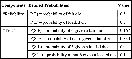
Consider that a fair die will land on each of its sides with roughly equal probability, 1/6 (16.7%). Therefore, landing on 6 would have a 1/6 probability and landing on anything but 6 would have a 5/6 probability. Perhaps one would estimate that the probability of a loaded die landing on 6 is 9/10 (90%) and the probability of it landing on anything else would be 1/10. Further, say that you have no certainty of whether the dice is loaded, it is 50/50 that it could be either. By throwing a die and observing the outcome (perhaps termed as a “test”), your confidence of the dice being loaded or not (which can perhaps be termed as the “reliability” of the dice) can be modified and improved. The prior information is shown in Table 7.2.

Now the die is thrown. Consider that the result is a 6. Using Bayes equation, the updated probability that the die is loaded can be found using the equation:

$P (L | S) = \frac{P (S | L) P (L)}{P (S | L) P (L) + P (S | F) P (F)} = \frac{0.9 \times 0.5}{0.9 \times 0.5 + 0.167 \times 0.5} = 0.843$ $P (L | S) = \frac{P (S | L) P (L)}{P (S | L) P (L) + P (S | F) P (F)} = \frac{0.9 \times 0.5}{0.9 \times 0.5 + 0.167 \times 0.5} = 0.843$

(7.26)

Table 7.2

Initial Values for the Die Roll Example

Components	Defined Probabilities	Value
“Reliability”	P(F) = probability of fair die	0.5
“Reliability”	P(L) = probability of loaded die	0.5
“Test”	P(S\|F) = probability of 6 given a fair die	0.167
	P(S′\|F) = probability of not 6 given a fair die	0.833
	P(S\|L) = probability of 6 given a loaded die	0.9
	P(S′\|L) = probability of not 6 given a loaded die	0.1

And the updated probability that the die is fair is simply the complement of 0.843 by the law of total probability, which is 0.157. This initial test makes the die seem as though it is probably loaded. But more testing can be done by using the posterior distribution as the new prior and throwing the die again. Say the result of the second throw is a 2. What are the chances the die is loaded after two data points?

$P (L | S′) = \frac{P (S′ | L) P (L)}{P (S′ | L) P (L) + P (S′ | F) P (F)} = \frac{0.1 \times 0.843}{0.1 \times 0.843 + 0.833 \times 0.157} = 0.392$ $P (L | S′) = \frac{P (S′ | L) P (L)}{P (S′ | L) P (L) + P (S′ | F) P (F)} = \frac{0.1 \times 0.843}{0.1 \times 0.843 + 0.833 \times 0.157} = 0.392$

(7.27)

And the updated probability of a fair die is the complement at 0.608. By using the prior probability as our new guess and scaling it by the likelihood that the roll would not be a 6, we have come up with a much more optimistic guess of whether the die is loaded.

This example may seem trivial, but by relating a loaded die to reliability and rolling to testing, it can be seen how this approach may be useful in the case of a process plant. Say, instead of a loaded die, a plant has a tank that has a chance of a defect due to corrosion, and instead of rolling a die to test, several small samples are taken at various intervals to perform corrosion tests. Continuous testing and updating through the Bayes theorem can identify trends in important fields such as reliability as simply as it can predict whether dice are loaded.

7.2.2.3. Bayes theorem and application to equipment failure

Bayes theorem can also be extended to a continuous form where probability distributions are used:

$f ″ (θ | x) = \frac{P (x | θ) f' (θ)}{\int_{- \infty}^{\infty} P (x | θ) f' (θ) d θ}$ $f ″ (θ | x) = \frac{P (x | θ) f' (θ)}{\int_{- \infty}^{\infty} P (x | θ) f' (θ) d θ}$

(7.28)

where f′ represents the prior probability distribution, f″ represents the posterior probability distribution, and P(x|θ) is the probability of x as a function of θ. The idea is the same: update prior beliefs about the performance of the system with observed information, but in this case probability distributions are used and updated.

Typically, the selection of the prior distribution is somewhat subjective, so a selection of a conjugate prior from the same family of distributions as the posterior can make the choice more objective for easier computation of the posterior parameters. An example of conjugate distributions are a beta prior and binomial likelihood (leading to a beta posterior), and a gamma prior and Poisson likelihood (leading to a gamma posterior). According to the literature (Shafaghi, 2008), the gamma distribution and Poisson likelihood are best suited to finding a failure rate of components, while the binomial likelihood and beta distribution are best suited for the calculation of rate of failure on demand. Explanation of the Poisson/gamma process follows.

The discrete Poisson distribution assumes that events of interest are randomly dispersed in time or space with a constant intensity of λ (Modarres et al., 2009). The distribution can be expressed as:

$P (x) = \frac{ρ^{x} \exp (- ρ)}{x!}$ $P (x) = \frac{ρ^{x} \exp (- ρ)}{x!}$

(7.29)

where x is a discrete variable that describes the number of events observed at a certain time interval, and ρ = λt, where λ is as described earlier and t is the time interval of interest. The Poisson distribution can be used as the likelihood function gathered from observed data in the continuous Bayes formulation.

The gamma distribution is the continuous analog of the Poisson, and models time for α events to occur randomly with an observed mean time of β between events. This is used as the prior probability in the continuous Bayes formulation. This distribution can be expressed as:

$f (t) = \frac{1}{β^{α} Γ (α)} t^{α - 1} \exp (- \frac{t}{β})$ $f (t) = \frac{1}{β^{α} Γ (α)} t^{α - 1} \exp (- \frac{t}{β})$

(7.30)

Γ(α) can be simplified to (α – 1)! for all discrete values of α. As a simple example of the use of this continuous formulation, consider a set of tanks that are believed to crack due to corrosion in a gamma-distributed manner. It is believed that three events will occur randomly with a mean time or 5 years in between each event (α = 3, β = 5). The prior probability function can be stated as:

$f (t) = \frac{1}{5^{3} (3 - 1)!} t^{3 - 1} \exp (- \frac{t}{5}) = \frac{1}{250} t^{2} \exp (- \frac{t}{5})$ $f (t) = \frac{1}{5^{3} (3 - 1)!} t^{3 - 1} \exp (- \frac{t}{5}) = \frac{1}{250} t^{2} \exp (- \frac{t}{5})$

(7.31)

Suppose that the tanks are observed for 1 year and an event occurs. The observed λ value would now be one per year. The Poisson distribution of this observation would be:

$P (x) = \frac{{(1 \times t)}^{1} exp (- 1 \times t)}{1!} = t exp (- t)$ $P (x) = \frac{{(1 \times t)}^{1} exp (- 1 \times t)}{1!} = t exp (- t)$

(7.32)

Using the above formula to calculate the posterior distribution, we find:

$f ″ (θ | x) = \frac{P (x | θ) f' (θ)}{\int_{- \infty}^{\infty} P (x | θ) f' (θ) d θ} = \frac{t exp (- t) \cdot \frac{1}{250} t^{2} exp (- \frac{t}{5})}{\int_{0}^{\infty} t exp (- t) \cdot \frac{1}{250} t^{2} exp (- \frac{t}{5}) d t}$ $f ″ (θ | x) = \frac{P (x | θ) f' (θ)}{\int_{- \infty}^{\infty} P (x | θ) f' (θ) d θ} = \frac{t exp (- t) \cdot \frac{1}{250} t^{2} exp (- \frac{t}{5})}{\int_{0}^{\infty} t exp (- t) \cdot \frac{1}{250} t^{2} exp (- \frac{t}{5}) d t}$

(7.33)

this can be simplified to:

$f ″ (θ | x) = \frac{t^{3} exp (- \frac{6 t}{5})}{\int_{0}^{\infty} t^{3} exp (- \frac{6 t}{5}) d t} \approx \frac{1}{2.89} t^{3} exp (- \frac{6 t}{5})$ $f ″ (θ | x) = \frac{t^{3} exp (- \frac{6 t}{5})}{\int_{0}^{\infty} t^{3} exp (- \frac{6 t}{5}) d t} \approx \frac{1}{2.89} t^{3} exp (- \frac{6 t}{5})$

(7.34)

which fits the gamma distribution with parameters α = 4 and β = 5/6. The beta parameter has gone from a prediction of a mean time between events of 5 years and 10 months. The updated distribution compared with the prior distribution is as follows (Figure 7.2).

As can be seen, the probability of a failure has gone from relatively uncertain to having a significant spike early in operation as a result of the early failure. The Bayes model has predicted that the failures are expected to occur much earlier than originally expected. With further monitoring and continuous testing, it is possible that the model can once again be updated with more information as the time goes on to provide an even more accurate distribution.

Figure 7.2 Probability distribution function of tank failure.

7.2.2.4. Sources of generic data

Generic data may be obtained from a large number of sources, including CCPS Guidelines for Process Equipment Reliability Data (CCPS, 1988), IEEE Standard 500 – Guide to the Collection and Presentation of Electrical, Electronic, Sensing Component, and Mechanical Equipment Reliability Data for Nuclear-Power Generation Stations (IEEE, 1984), and the Offshore Reliability Data Handbook (OREDA, 2002). Further sources may be found in Lees' Loss Prevention in the Process Industries (Mannan, 2013).

7.2.3. Risk Assessment of LNG Terminals Using the Bayesian–LOPA Methodology

LNG refers to natural gas converted into its liquid state by super cooling to 260 °F (162.2 °C). LNG consists of 85–98% methane and the remaining is made up of smaller concentrations of heavier hydrocarbon components. LNG provides a cost-effective containment as well as transportation across great distances onshore and offshore at atmospheric pressure. Moreover, LNG is environmentally friendly because of its clean burning.

Because of these properties, the LNG demand has been growing to diversify the energy portfolios and fulfill the energy demand for LNG fuel for many applications, including heating, cooking, and power generation. Following the increasing demand for LNG, there are at least 100 currently active LNG facilities across the United States, including importation terminals, peak-shaving facilities, or base load plants. In addition, there are also a number of proposed projects for LNG terminals in North America. This analysis will focus on LNG terminals.

Even though LNG has several advantages, it may cause fire or explosion when it is discharged at undesired conditions. Especially in LNG terminals, large consequences may occur due to the huge amounts of LNG stored. Although the LNG industry has had an excellent safety record over the past 40 years, the risk related to LNG terminals may be increasing with the growing LNG industry. Consequently, risk-informed decisions found on sound science are critical to controlling risks related to LNG terminals.

In order to control risk, it is necessary to quantify the risk by applying a risk assessment methodology. LOPA provides a straightforward and systematic approach to obtain quantified risk results with less effort and time than other methods, especially QRA.

For the application of LOPA methodology, failure data of equipment and facilities are required to quantify the risk. However, the LNG industry has a relatively short operational history compared to other industries, such as the chemical industry, and there are only a few incident records. Therefore, available plant-specific failure data of LNG system are very sparse. The risk values estimated with these insufficient data may not show statistical stability or represent specific conditions of an LNG facility. Generic failure data from other industries such as the petrochemical and nuclear industries may be used for the LNG industry because they have sufficient and longer-term historical records. However, these data also may not provide appropriate risk results for the LNG industry because the operational conditions and environment of LNG facilities are different from those of other industries.

Therefore, the Bayesian estimation can be used to obtain more reliable risk values. Bayesian logic can produce updated failure data using the prior information of generic data from other industries and the likelihood information of LNG plant-specific data. The updated data can reflect both statistical stability from the generic data and the specific conditions from the LNG plant data. In addition, Bayesian estimation includes variability and uncertainty information to result in Bayes credibility or probability intervals, such as a 90% credible interval of updated data, even though LNG plant failure data are sparse. In other words, the weakness of failure data from the LNG industry can be reduced or overcome by the use of Bayesian estimation. Therefore, the Bayesian–LOPA methodology, which was newly developed in this paper, was used to conduct risk assessments for an LNG terminal.

7.2.3.1. Methodology development

LOPA is a simplified form of QRA that uses initiating event frequency, consequence severity, and the probability of failure on demand (PFD) of independent protection layers (IPLs) to estimate the risk of an incident scenario (Crowl, 2001). Typically, LOPA builds on the information developed during process hazard analysis (PHA) where techniques, such as HAZOP and What-If methods, are used to develop incident scenarios. The purpose of LOPA is to estimate risk values for a facility so that risk decisions can be made based on tolerable risk criteria adopted by the facility. LOPA can also be used to rank the estimated risk values of identified incident scenarios to give priority to safety measures for higher-risk scenarios and for critical equipment that contribute significantly to the risk levels.

The Bayesian–LOPA methodology is an advanced LOPA method, because it can yield more statistically reliable or concrete risk results in an LNG facility than normal LOPA methods. Figure 7.3 shows the procedure of the Bayesian–LOPA method.

As a PHA method, a hazard and operability (HAZOP) study (Crowl and Louvar, 2001) will be used because it is one of the most systematic hazard identification methods. The HAZOP method requires process information such as piping and instrumentation diagrams (P&IDs) and process flow diagrams, which include basic designs and minimum specifications adopted from industrial standards such as NFPA 59A (NFPA, 2006) and EN 1473 (Committee of European Nations, 1997) for an LNG terminal. Results from an HAZOP study are used to make incident scenarios, which can be pairs of causes and consequences. The incident scenarios are screened according to severity by the category method, which is a qualitative way to classify consequences using engineering expert judgment.

Figure 7.3 Procedure for the Bayesian–LOPA method.

Causes found in the HAZOP results may be initiating events of incident scenarios. After identifying an initiating event, its occurrence frequency should be obtained for a LOPA application. Based on Bayesian estimation, the frequency of an initiating event can be obtained by using a conjugate gamma distribution for the prior information and a Poisson distribution for the likelihood function as shown in Figure 7.4. Offshore reliability data (OREDA) (OREDA, 2002) can be used in this manner as prior information, because data were produced from a gamma distribution. Figure 7.5 also shows some formulas for not only gamma and Poisson distributions, but also mean value and 90% credible interval of Bayesian-updated posterior values. If there is no prior information, the Jeffreys noninformative prior (Jeffreys, 1961) may be used. For the plant-specific likelihood information, the LNG plant failure database (Johnson and Welker, 1981), which was established from 27 LNG facilities, is used. This database provides operating hours, number of failures, and mean time between failures (MTBFs) of equipment or facilities.

After obtaining the frequency data of an initiating event, it is necessary to identify each independent protection layer (IPL), which can be found and chosen in the list of safeguards of each incident case in the HAZOP results. However, even though all IPLs can be safeguards, not all safeguards are IPLs, because IPLs must meet the three requirements: independence, effectiveness, and auditability. Thus, very careful consideration should be given to designate a safeguard as an IPL. Following IPL identification, the PFD of each IPL should be obtained. Generally, this procedure is similar to the case of initiating events, but there are a few differences in the distributions and mathematical calculations. The PFDs of IPLs can be estimated using the conjugate beta prior distribution and binomial likelihood distribution, as shown in Figure 7.4. (Table 7.3)

EIReDA (European Industry Reliability Data Bank) (Procaccia et.al., 1997) is used for prior information, because it was prepared from a beta distribution. When EIReDA does not provide failure data, the newly developed frequency–PFD conversion method (Yun, 2007) may be used. LNG plant failure data will be represented by a binomial likelihood function. However, even though some types of failure data are available, the EIReDA database does not provide the number of demands, which is needed together with the number of failures for the binomial distribution. The number of demands can be estimated, however, by correlation using the PFD estimating equation as shown in Figure 7.5, provided periodic tests of equipment are performed that reveal the failures (Crowl and Louvar, 2001; Yun, 2007).

The next step is to use a spreadsheet to calculate the frequency of an incident scenario from the equation given in the “Estimate scenario frequency” step of Figure 7.3. Microsoft EXCEL software can be used to create the spreadsheet.

The last step is to make risk decisions from comparison of an obtained scenario frequency with the tolerable risk criteria, which may be specified by companies, industries, or government. If the estimated frequency cannot meet the tolerable criteria, some recommendations that may include additional IPLs or more frequent proof tests must be given to reduce the incident frequency or mitigate the severity of consequence. As shown in Figure 7.3, these steps will be repeated for every incident scenario. The frequencies of all incident scenarios is estimated and then compared to each other to rank the risks among all scenarios with similar consequence severities. This risk ranking may be used also to develop strategies for maintenance or safety measures.

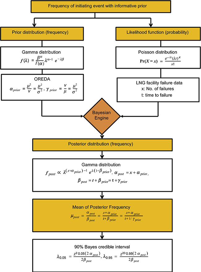
Figure 7.4 Schematic diagram of Bayesian estimation for IPLs.

Figure 7.5 Schematic diagram of Bayesian estimation for initiating events.

Table 7.3

LOPA Incident Scenarios in an LNG Terminal

No.	Scenarios
1	LNG leakage from loading arms during unloading.
2	Pressure increase of unloading arm due to block valve failure closure during unloading.
3	HP pump cavitation and damage due to lower pressure of recondenser resulting from block valve failed closure. Leakage and fire.
4	Higher temperature in a recondenser due to more boils off gas (BOG) input resulting from flow control valve spurious full open. Cavitation and pump damage leading to leakage.
5	Overpressure in tank due to rollover from stratification and possible damage in tank.
6	LNG level increases and leads to carry over into the annular space of LNG, because operator lines up the wrong tank. Possible overpressure in tank.
7	Lower pressure in tank due to pump-out without BOG input resulting from block valve failed closure. Possible damage tank.

7.3. Multiscale Models

Modeling failure mechanisms is important for predicting the future performance of materials in a system. Failure data from past incidents alone are not sufficient by itself in predicting material failure, due to process changes and changes in the microstructure of materials with time (Taylor, 2015). The mechanical deformation and material failure of many engineering materials are inherently multiscale in nature (Curtin and Miller, 2003). Given that, multiscale materials modeling have been proved to be a powerful approach in combining knowledge from historical data, experimental results, and first principle-based calculations for predicting the risk of material failure. However, model development for material degradation or failure using all available information and underlying fundamental physics is a challenging problem. In addition to addressing material failure, development of models should also incorporate abilities to assess various risk mitigation strategies. One such example could be the addition of corrosion inhibitors for corrosion issues as illustrated in the later part of this chapter. Among several set of modeling approaches in addressing material failure problems, atomistic and quantum mechanics–based simulations stand out as the most fundamental class of modeling approaches. While the failure of material at the macroscale happens at a very different time and length scale than that can be modeled at the atomistic level, the underlying physics between the two events are connected, albeit sometimes in a nonobvious fashion. It is well established that processes governing observed macroscopic material behavior occur at various time and length scales (Curtin and Miller, 2003). At the nanoscale, the origin of failure may initiate from the nonuniform distribution of the electrons (Sih, 2005, 2008). Examples of defects at the nanoscale include vacancies, impurities, dislocations, voids, crack tips, and grain boundaries. There is an intimate coupling between the disparate length scales as the long-range defect stress fields can introduce nucleation of new defects at the atomistic scale (Curtin and Miller, 2003). The collective effect of plethora of defects interacting at the atomistic level translates into material's macroscopic response to external forces. Fidelity of the mathematical model developed for describing a failure mechanism can be improved by incorporating details from multiscale methods. Fully atomistic simulation of most collective defect processes is not feasible due to the requirement of simulating a large number of atoms.

7.3.1. Material Failure

Owing to its inherent multiscale nature, phenomena such as fracture are best studied through application of coupled multiscale models. Figure 7.6 depicts the fracture phenomenon at various characteristic length scales.

Typically, multiscale methods in modeling material failure require modeling at the quantum mechanical, atomistic, and finite element analysis level. While detailed molecular-level interactions are dealt at the quantum and atomistic simulation level, finite element analysis allows one to model defects at the continuum level. Accurate estimation of energetics lies at the core of the model development for material failure. In theory, atomistic simulation should be able to accurately estimate zero energy positions of the atoms constituting the material of interest. Estimation of potential energy of a system can be done by performing quantum mechanical calculations or by using a suitable force field for the system of interest as discussed in Chapter 3.

The response of a material to an external stress is governed by its stiffness constants. By applying the formal definition in Voigt notation, the elastic stiffness matrix can be represented as:

$C_{i j} = \frac{1}{V_{0}} \frac{\partial^{2} E}{\partial ε_{i} \partial ε_{j}}$ $C_{i j} = \frac{1}{V_{0}} \frac{\partial^{2} E}{\partial ε_{i} \partial ε_{j}}$

where C_ij is the elastic constant, E is energy, and ε_i is the strain in the ith direction. Performing Taylor series expansion of energy around minimized structure as a functional form of the strain, ε, energy of a system can be represented as:

$E (ε) = E_{0} + \sum_{i = 1}^{6} {(\frac{\partial E}{\partial ε_{i}})}_{E_{0}} ε_{i} + \frac{1}{2} \sum_{i, j = 1}^{6} {(\frac{\partial^{2} E}{\partial ε_{i} ε_{j}})}_{E_{0}} ε_{i} ε_{j + \dots}$ $E (ε) = E_{0} + \sum_{i = 1}^{6} {(\frac{\partial E}{\partial ε_{i}})}_{E_{0}} ε_{i} + \frac{1}{2} \sum_{i, j = 1}^{6} {(\frac{\partial^{2} E}{\partial ε_{i} ε_{j}})}_{E_{0}} ε_{i} ε_{j + \dots}$

where E₀ refers to the energy of zero–strain equilibrium configuration. Since the force on the atoms of a molecular structure in its energy minimized configuration is zero, neglecting the higher order terms in the Taylor series expansion, the elastic constant C_ij can be estimated by implementing molecular-level modeling approaches. Figure 7.7 depicts a typical outcome of energy–strain curve as estimated based on energy minimization of a molecular system under a given strain either through quantum mechanics or molecular mechanics-based approach. Fitting the curve will estimate the elastic constant of interest.

Figure 7.6 Characteristic length scale associated with material fracture.

In general, the steps involved are:

• Define the unit cell of the system of interest

• Choose a suitable classic force field with modified interaction potential as applicable

• For various values of strains, estimate the energy of the unit cell and express it in terms of strain

• Use the expression,

C_{i j} = \frac{1}{V_{0}} \frac{\partial^{2} E}{\partial ε_{i} \partial ε_{j}}

$C_{i j} = \frac{1}{V_{0}} \frac{\partial^{2} E}{\partial ε_{i} \partial ε_{j}}$

, as mentioned before in the Taylor series expansion for estimation of the elastic constants

At the continuum level, the potential energy of a system can be estimated as:

$E = \int_{V} W (x) d V$ $E = \int_{V} W (x) d V$

where E is the potential energy and can be estimated through integrating W(x), the energy density at location x, over the total volume V. The energy density can be defined as:

Figure 7.7 Typical energy–strain curve of a system.

$W (x) = \frac{1}{2} (C_{i j} \cdot ε_{i j})$ $W (x) = \frac{1}{2} (C_{i j} \cdot ε_{i j})$

The value of C_ij can be obtained from experimental or molecular modeling approaches. In a similar fashion, at the continuum level, finite element analysis is implemented for estimation of the strain field of a deformed body due to application of external forces (Curtin and Miller, 2003). The minimization of energy of a given system under external forces allows one to estimate the strain field. At the continuum level the energy equation can be rewritten in terms of the elements in the finite element analysis approach:

$E = \sum_{i}^{n} E_{i}$ $E = \sum_{i}^{n} E_{i}$

$E_{i} = \int_{V_{i}} W_{i} (x) d V_{i}$ $E_{i} = \int_{V_{i}} W_{i} (x) d V_{i}$

where E_i is the energy of the ith element, V_i is the volume of the ith element, and W_i(x) is the strain energy density at location x at the ith element.

At each node, displacement due to deformation is calculated. Deformation between nodes can be calculated through shape functions or interpolation functions. Accordingly, the displacement of a point within an element depends only on the displacement of the two nodes corresponding to the vertices of the element. The energy is minimized with respect to the nodal degrees of freedom. The strain energy density, W_i(x), can be written as:

$W_{i} (x) = W_{i} (F (x))$ $W_{i} (x) = W_{i} (F (x))$

where F(x) is the deformation gradient, the fundamental quantity of continuum deformation. For material with no defects, the deformation gradient can be assumed to be homogeneous. Homogeneous deformation gradient in a crystal can be calculated using molecular modeling approaches either through classic force field-based approaches or through quantum mechanical calculations by implementing the Cauchy–Born rule (Weiner, 2012; Ericksen, 2008). For crystals, the Cauchy–Born rule is effective in correlating the deformation energy at the continuum level to atomistic potential energy from stretched crystals at the atomistic level. The rule states that the atomistic positions within the crystal lattice follow the overall strain of the medium and that it does not allow relaxation of the lattice atoms within the unit cell. Accordingly, it must be borne in mind that the Cauchy–Born rule is only valid for small deformations. Figure 7.8, illustrates the deformation of a crystal from atomistic and continuum viewpoints (Buehler, 2008). At the atomistic level, one is interested in shifting of the individual atoms, whereas at the continuum level, it is the overall deformation resulting in a strain field within the macroscopic body.

One of the challenges in multiscale model development of material failure through atomistic simulation and finite element analysis lies in the formulation of the strain energy density functional (Curtin and Miller, 2003). The true atomistic energy is nonlocal, whereas at the continuum level, the deformation around an element is assumed homogeneous. Owing to the scale difference, at the finite element level it is not possible to represent the true inhomogeneous deformation representation as assessed by atomistic simulation. One approach to address this is through implementation of homogeneous deformation within an element consisting of several nodes, each represented by an atom, to estimate the approximate atomic positions in the deformed body. While the resultant atomic positions, represented by nodes, will only be approximate, the continuum strain energy density calculated in this approach corresponds to an atomistic calculation of the energy for the approximate set of atom positions. Thus the deformation at the continuum level accounts for the nonlocal and finite range-interatomic potentials with an approximation to the actual atomic positions. For achieving equilibrium, the energy estimated in this approach needs to be minimized with respect to the nodal degrees of freedom. In order to estimate the energies for displacement of the nodes, it must be taken into account that, in a finite element analysis, a change in the position of a node affects the deformation gradient of all the elements connected to it.

Figure 7.8 Deformation of a crystal. (a) atomistic viewpoint, (b) continuum viewpoint (Buehler, 2008).

For an integrated coupled model, the idea is to use atomistic-level description at regions where details are important and continuum descriptions in other regions as illustrated in Figure 7.9.

Approximations are necessary while formulating a problem in this manner due to the fundamental incompatibility between atomistic and finite element analysis approach as noted before. The “pad” region in Figure 7.9 consists of pseudo atoms and overlaps physical space with the mesh of the finite element analysis approach. At the interface, there is a one-to-one mapping between atoms and nodes from mesh of the finite element approach. Various approaches (Miller et al., 1998; Shenoy et al., 1998; Rudd and Broughton, 2000; Kohlhoff et al., 1991; Shilkrot et al., 2002; Buehler, 2008; Ersland et al., 2011) exist to couple the two modeling approaches at the transition region lying between the atomistic and the continuum region. Instead of delving deeper into these topics, the goal here is to make the reader aware of various detailed and coupled modeling approaches that can be implemented in understanding and estimating characteristics of material failure. Owing to the scale of deformation, often an all-atomistic model is not feasible in today's date and hence one can consider the coupled multiscale modeling approach as an alternative that can provide significant insight using reasonable amount of resources. There are also studies involving only molecular dynamics to investigate the effect on structural properties of steel such as effect of grain boundary sliding on the toughness of steel (Xie et al., 2013). Grain boundaries are defects in crystal structures and lies at the interface between two crystallites. Implementing molecular dynamics, the work could assess the crack propagation dynamics with time as depicted in Figure 7.10.

Figure 7.9 Atomistic finite element analysis-based coupled multiscale modeling approach.

A similar problem has also been addressed by coupling atomistic and finite element analysis (Park et al., 2005) in a similar way discussed before.

The formation and breaking of covalent bonds at and in the vicinity of the crack tip can be addressed by a quantum mechanical approach or tight binding formulation. The region somewhat further away from the crack tip, may experience large strain but is not expected to result in formation or breaking of bonds. Hence, these regions can be treated through interatomic potentials in a classic force field. Even further, the strain fields tend to become homogeneous and the strain gradients are small. Hence, a continuum finite element analysis is appropriate for the far-field region. With three different modeling approaches, two interfaces show up. The interface between finite element and molecular dynamics has been discussed before. The FE mesh dimensions are brought down to atomistic dimensions prior to switching over to the atomistic simulation domain. The second interface lies between the atomistic and tight binding/quantum mechanical calculations. Given that this interface is in the vicinity of the crack, it is more dynamic in nature and complex to model. However, modeling methods have been developed to tackle such challenges on a system-by-system basis and is nontrivial in nature (Buehler, 2008). Using ReaxFF force field is another possible approach where one can address an atomistic-level phenomenon of both reactive and nonreactive atoms.

The fracture response of materials is inherently linked to process safety incidents. For example, fracture response of pipelines subject to large plastic deformation is of interest when looking into designing long-distance offshore pipelines (Østby et al., 2004; Jayadevan et al., 2003). This chapter introduces the readers to the existing model development approaches incorporating detailed atomistic studies that can be used in simulating these processes (Buehler, 2008). The details discussed here are merely an outer layer of the topic but should provide an idea about the immense potential of multiscale modeling methods in assessing fracture and deformation characteristics of material under various process conditions. Further readings, such as the book by Buehler (2008), are suggested.

Figure 7.10 (a–c) Crack propagation as estimated by implementing MD studies on ultrafine grain structure steel (Xie et al., 2013).

7.3.2. Corrosion

Among various failure mechanisms, equipment or pipeline failure from corrosion resulting in process safety incident is a very likely phenomenon (Fire, 2012). Accordingly, corrosion monitoring and corrosion control are of substantial importance in the process industries. Corrosion control can involve any or all of the following major approaches (Center for Chemical Process Safety [CCPS], 2012):

• Change in materials

• Change in the process environment

• Change in process conditions

• Addition of corrosion inhibitors

• Use of barrier linings or coatings

• Application of electrochemical techniques

In all of these changes, one needs to understand the sensitivity of the corrosive action with respect to the change(s) introduced.

Addition of corrosion inhibitors to the process fluid requires understanding of the underlying mechanism of its action. Their classification according to the mechanism of their action is provided in Table 7.4 (Center for Chemical Process Safety [CCPS], 2012).

Quantum mechanical approaches have been proved to be a powerful tool for studying the structure and behavior of corrosion inhibitors (Gece, 2008). The idea is to assess the efficiency of corrosion inhibitors, through implementing molecular modeling studies on those chemicals with a desired set of properties. In the case of organic inhibitors, the inhibition mechanism is dictated by physicochemical and electronic properties of the inhibitor. The combined effect of the facts that a molecular system can be characterized solely based on its molecular structure and that chemical reactivity of a set of molecules will account for any inhibitor mechanism of interest enables one to use molecular modeling approaches as powerful tools in corrosion inhibitor studies.

Upon performing quantum chemical calculations on corrosion inhibitors, the approach is to discover a strong correlation between the inhibition mechanism and a quantum chemical parameter. Once that is determined, one can assess the effect of inhibitors by monitoring the quantum chemical parameter. Quantum chemical parameters can be atomic charges, atomic energies, molecular orbital energies, and dipole moment. The usual steps in estimating these parameters start with geometry optimization including calculation of atomic charges, similar to any quantum mechanical calculation as illustrated in Chapter 3. Further studies are only performed with the already optimized molecular structure of the system of interest.

Semiempirical calculations to assess the effectiveness of imidazole derivatives as acidic corrosion inhibitors for zinc and iron have been performed using AM1, PM3, MNDO, and MINDO/3 methods by Bereket et al. (2000, 2001). Several quantum chemical parameters such as total energy, atomic charges, ionization potential, dipole moment, HOMO (highest occupied molecular orbital), and LUMO (lowest unoccupied molecular orbital) energies were calculated.

In a similar manner, El Issami et al. (2007) showed that less negative HOMO energy along with a smaller energy gap between HOMO and LUMO indicated greater inhibitor efficiency. Inhibition efficiency can be estimated in several ways including using change in current densities and polarization resistance. For example, for a 100% efficient inhibition, the current density measured should be negligible or close to zero. Figure 7.11 illustrates the correlation found in the study between inhibition efficiency, determined through experiments, and HOMO energies for three different systems with the corresponding inhibitors.

Table 7.4

Corrosion Inhibitors (Center for Chemical Process Safety [CCPS], 2012)

Inhibitor	Method of Action	Example
Absorption type	Suppresses metal dissolution and reduction reactions	Organic amines
Hydrogen evolution poison	Retards hydrogen evolution but can lead to hydrogen embrittlement	Arsenic ion
Oxygen scavenger	Removes oxygen from aqueous solution including water	Sodium sulfite, hydrazine
Oxidizer	Inhibits corrosion of metals and alloys that demonstrate active–passive transition	Chromate, nitrate, and ferric salts
Vapor phase	Blanket gas for machinery or tightly enclosed atmospheric equipment	Nitrogen blanket

Figure 7.11 Correlation between HOMO (E_HOMO) energy and inhibition efficiency (E_M) for three (AT, DTA, and ATA) scenarios.

In addition to using quantum mechanical methods, molecular dynamics approaches have also been used to investigate corrosion phenomena (Susmikanti et al., 2012). The study looked into the effect of increasing molybdenum (Mo) content in steel with the objective of increasing corrosion resistance. Since a molecular dynamics approach was used, the effect of temperature was also investigated. A visual approach showed increase of corrosion with increasing temperature and increase of corrosion resistance with increasing Mo percentage. Figure 7.12 illustrates the increase of corrosion rate for change in temperature as can be observed by inspecting the surface (depicted by the dark line inside the rectangular box at the interface) between crystal steel-containing Mo (left) and coolant material Pb-Bi (right).

Figure 7.12 Corrosion characteristics for steel with Mo 2–3% content at 773 K (top) and 1373 K (bottom).

Computational chemistry can be used as a powerful tool for corrosion inhibitor studies. Both quantum mechanical calculations and molecular dynamics study can be implemented in assessing inhibitor efficiency, corrosion resistance, and potential to corrosion studies. While experimental studies are needed for validation, computational-chemistry approaches can narrow down the number of experimental studies required in a significant way.

Sync Reading Stream

What's this?

..................Content has been hidden....................

You can't read the all page of ebook, please click here login for view all page.

Table of Contents for 7.1. Introduction

Create new playlist

Sign In

Sign Up

Abstract

Keywords

7.1. Introduction

7.2. Failure Rates for Various Types of Equipment

7.2.1. Examining Extrapolation of Current Data Outside Their Applicable Domain of Certain Temperature and Pressure Failure Rate of Equipment

7.2.1.1. Mean time to failure

7.2.1.2. Exponential distribution

7.2.1.3. Gamma distribution

7.2.1.4. Weibull distribution

7.2.1.5. Normal distribution

7.2.1.6. Lognormal distribution

7.2.1.7. Failure rates without failure

7.2.2. Bayesian Logic

7.2.2.1. Introduction to the Bayes theorem

7.2.2.2. An illustrative example of Bayes theorem

7.2.2.3. Bayes theorem and application to equipment failure

7.2.2.4. Sources of generic data

7.2.3. Risk Assessment of LNG Terminals Using the Bayesian–LOPA Methodology

7.2.3.1. Methodology development

7.3. Multiscale Models

7.3.1. Material Failure

7.3.2. Corrosion

Table of Contents for
7.1. Introduction