4.4. Explosion Modeling
CFD explosion modeling is focused on the understanding of possible consequences from large-scale industrial accidental events such as VCE, BLEVE, DDT, and dust explosion. Besides data regarding overpressures and impulse generated from these types of explosion, which is also the main hazards of explosion in context of process safety, CFD simulation results provide extensive information regarding the development of flammable clouds, the movement of flame and pressure waves, and the interaction between the pressure wave and the obstacles. These data are critical for the design, layout, control, and mitigation of explosion hazards. Even though the four phenomena described in this section are all related to explosion and pose the same type of hazards, their explosion kinetics and mechanism, temporal and spatial scales, and involved geometries are significantly different in terms of CFD simulation; thus, they will be covered in separated sub-sections below.
4.4.1. Vapor Cloud Explosion
The main advantage of CFD in simulating VCEs is its capability to accurately represent complex geometries to a detailed level. This capability is critical in studying VCE, because it is well known that obstacles have significant effects on the development of flammable cloud and VCE strength (e.g., the overpressure magnitude and affected radii). The interaction of gas flow with obstacles generates turbulence, which increases the energy release rate and the flow velocity of the combustion process and further intensifies the turbulence ahead of the flame. This feedback cycle increases the flame acceleration and strengthens the overpressure generated from VCE. This requires very accurate representation of all geometrical features, making CFD a clear advantage over simpler models in the capability of simulating VCEs in complex geometries.
Besides providing predictions regarding the development of flammable cloud, overpressure magnitude, and affected radii, CFD simulations are conducted to gather comprehensive information on the effects of overpressures on structural members, the possible arrangement of explosion vents, the effectiveness of protective barriers, and other mitigation measures.
4.4.1.1. Geometry representation
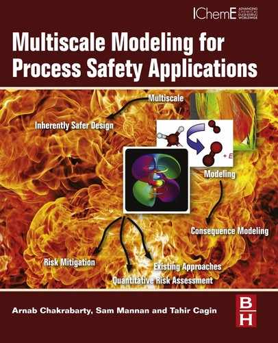
To take full advantage of a CFD simulation in VCE, there needs to be a detailed and accurate geometry representation. However, practically for large-scale simulation in a typical process facility (e.g., a refinery, a chemical plant, or an offshore platform), there are multiple obstacles including tube pipe bundles, structural trusses, and pieces of process plant equipment, and surrounding environmental objects such as trenches and trees (Bakke et al., 2010), whose numbers can be up to several thousand with dimensions ranging in several orders of magnitude (millimeters to meters). This reality makes geometry representation one of the most challenging aspects of using CFD in a VCE study for an actual industrial facility. A relatively simple approach using a Cartesian grid with porosity distributed resistance (PDR) (Patankar and Spalding, 1974) is a popular concept used in many CFD codes such as FLACS, AutoReaGas, and EXSIM (see Figures 4.19 and 4.20) (Lea, 2002; Cant et al., 2004; Baraldia et al., 2009).
Detailed and accurate geometry representations of large-scale industrial facilities as presented in Figure 4.19 are critical in CFD simulation of VCE. The Cartesian/PDR approach was invented in order to present large-scale complex geometries by dividing them approximately into resolved geometrical objects, often large objects whose dimensions could be represented in the grid, and unresolved geometrical objects, often smaller objects whose dimensions are smaller than the grid size. By that, the resolved geometries (e.g., large objects) are treated explicitly on a computational grid, whereas the unresolved geometries (e.g., small objects) are represented using the PDR method as area porosities on the control volume faces and as volume porosities within the control volume faces. The porosity is defined as the fraction of a face or volume available for fluid flow, as opposed to the blockage, which is the fraction blocked from access by the fluid. The flow resistance, turbulence, source-term, and the flame speed enhancement are then calculated using these defined porosities. In this way, complex geometries in oil and gas or chemical facilities such as pipe systems or skid mounted equipment can be divided into multiple parts and represented by PDR “sub-modules”, simple, primitive geometries such as isolated cylinders or square bars, fully developed tube-bundle flows, simple planar grids, and uniform porous surfaces or regions (Cant et al., 2004).

Figure 4.19 Rendering explosion modeling results from a CFD simulation for an offshore platform using FLACS. © FAO, 1988. In Vitro Toxicology. pp. 1–14. http://agris.fao.org/agris-search/search.do?recordID=US19890077884 (02.02.15.).
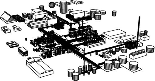
Figure 4.20 Graphic representation of the Flixborough plant for CFD simulation using EXSIM CFD code. Reproduced by permission with Hoiset et al. (2000).
Computational geometry can be prepared either by manually defining a set of primitives (boxes, cylinders, and planes) representing corresponding obstacles or automatically by importing from CAD drawings. Many, but not all, commercial CFD packages such as FLACS or AutoReaGas provide certain types of interface to convert CAD data into CFD 3D models (Lea, 2002; Cant et al., 2004). The process of defining all objects in large facilities such as refineries or offshore platforms requires an extremely large amount of time. This process can be sped up by using the current technology in laser 3D scanning to obtain the detailed information and converting the scanned data into CAD before importing into CFD codes.
The geometry representation on the CFD grid needs major improvement over the current Cartesian/PDR approach, which has been criticized for being unable to accurately and completely represent complex geometries (Lea, 2002). More recently, other more advanced methods have been explored to fully represent the interested geometries; for example, the unstructured body-fitting grid or the adaptive meshing has been successfully implemented in certain CFD codes (Fairweather et al., 1999; Lea, 2002; Cant et al., 2004; Baraldia et al., 2009).
4.4.1.2. Turbulence model
The two-equation k–ε turbulence model is the model of choice for all CFD codes for VCE simulations because it provides a reasonable balance between accuracy and computing cost (Lea, 2002). This model is based on the gradient transport assumption and the Boussinesq eddy dissipation turbulence model (Blazek, 2007). Other more advanced derivatives of the k–ε turbulence model such as the Reynolds normalization group (RNG) and the realizable k–ε turbulence model, as well as newer models such as Reynolds stress turbulence models have not been implemented in CFD codes for VCE modeling (Lea, 2002). The advanced LES methods such as the eddy viscosity LES and RNG-LES have been applied in hydrogen explosion study (Colin et al., 2000; Durand and Polifke, 2007; Baraldia et al., 2009; Lecocq et al., 2011).
The k–ε model was originally developed and validated for only certain fundamental nonreacting constant flow and has been shown that it may not be able to predict the large-scale turbulent reacting flow in a complex 3D geometry (Lea, 2002). Therefore, more research is needed on the application of turbulence models, such as exploring more advanced versions of the k–ε model and other turbulence model such as Reynolds stress model implementation in CFD codes for VCE studies.
4.4.1.3. Combustion model
Combustion model is used to calculate the combustion reaction rate in VCE events. Generally, it is reasonable to use a fast reaction assumption for premixed fuel–air mixtures in explosion modeling, thus allowing some simplification in combustion models needed. Available CFD codes use either prescribed reaction rates based on empirical correlations of burning velocity or the eddy break-up model (Magnussen and Hjertager, 1977), which requires a certain resolution of the flame front to work (Lea, 2002; Cant et al., 2004). The latter is used in commercial CFD codes such as EXSIM and CFX-4 models, while the former is used in AutoReaGas (Lea, 2002). Newer versions of FLACS and AutoReaGas use an eddy break-up–based combustion model called the “β transformed” gradient method for flame tracking with Bray's correlation for turbulent burning velocity (Bray, 1990; Arntzen, 1998; Durand and Polifke, 2007; Baraldia et al., 2009). These two simple approaches for modeling combustion are also used in newer and more sophisticated CFD codes such as COBRA (empirical), NEWT (eddy break-up), and REACFLOW (eddy break-up). The relatively new CREBCOM combustion model is implemented in CFD codes COM3D-3.4 and b0b (Efimenko and Dorofeev, 2001; Baraldia et al., 2009).
Other more combustion advanced models available are the laminar flamelet, probability PDF transport, and conditional moment closure; even though they have been developed and used in combustion studies for a long time, they have not been used in VCE CFD modeling (Vianna and Cant, 2010; Lecocq et al., 2011). Studies have been done to incorporate more detailed chemistry and advanced models into combustion models but only on a very small experimental scale (Vianna and Cant, 2010; Lecocq et al., 2011). However, the possibility of using those models in a real large-scale facility is still open for discussion.
4.4.1.4. Published validation studies
Many studies have been published to validate the capabilities of CFD code in a VCE. In here, the focus is on independent validation projects that allow unbiased evaluation of the accuracy of available CFD explosion models. Projects of this type include the Modeling and Experimental Research into Gas Explosions (MERGE) (Popat et al., 1996) and Extended Modeling and Experimental Research into Gas Explosions projects funded by EU, the Joint Industry Project on blast and fire engineering for top side structures phases 2 (JIP-2) (Lea, 2002), and the European Commission–funded Network of Excellence, “Hydrogen Safety as Energy Carrier” (Baraldia et al., 2009).
In the MERGE project sponsored by the EU, experiments were designed to have an extensive evaluation of important components of CFD codes for VCE modeling. This project has three distinctive phases (Popat et al., 1996; Lea, 2002):
• Phase 1: Evaluation of the submodels such as combustion, turbulence, etc. incorporated into CFD codes.
• Phase 2: Verification of the CFD explosion prediction against small- and medium-scale geometries.
• Phase 3: “Blind” prediction form the CFD code developed for the explosion overpressures in the large-scale MERGE geometries, which consisted of a regular cuboidal pipe array filled with a combustible gas mixture. The blind prediction is considered the most stringent and precise test because the modeling predictions have to be submitted before the actual experiments are conducted.
Four CFD codes were used in the MERGE project: COBRA, EXISM, FLACS, and AutoReaGas. Among them, EXISM, FLACS, and AutoReaGas all use Cartesian/PDR for geometry representation; only COBRA, which is considered an advanced CFD model, is able to handle both Cartesian and cylindrical polar/arbitrary hexahedral meshes. All four CFD codes use the two-equation k–ε turbulence model for the turbulent flow. Although the blind predictions from all four models were considered scattered in comparison to the experimental data, they were within the accuracy range generally expected from simple CFD codes.
The MERGE project was extended into the EMERGE project in which the four aforementioned CFD codes were further evaluated in many more experimental tests. The results indicate the participating CFD codes can give acceptable results for practical application, but further improvement is required.
The JIP-2 projects had both experimental and modeling parts. The experimental portion was aimed at providing a better understanding of the mechanism and affecting factors behind VCE and establish a large database for CFD model calibration. Similar to the MERGE and EMERGE projects, the modeling portion of the JIP-2 project has three phases but with different focuses (Lea, 2002):
• CFD code blind predictions on a given geometry (8 m wide).
• Using the experimental results from the test in geometry in phase 1 to tune the models and repredict the experimental result.
• CFD code blind predictions on a larger geometry (12 m wide).
Table 4.6
List of CFD Codes and Participants in the Exercise
| CFD Codes | Participants |
| FLACS | DNV, Det Norske Veritas AS, Norway |
| GXC, GexCon AS, Norway | |
| COM3D-3.4 | FZK, GmbH, Germany |
| (CREBCOM) | |
| AutoReaGas | HSL, Health And Safety Laboratory, UK |
| ReacFLOW | JRC, European Commission Joint Research Center, Institute for Energy, the Netherlands |
| B0b | KI, Research Center Kurchatov Institute, Russia |
| FLUENT | UU, University of Ulster, UK |

Results from this JIP-2 project indicate that certain models were sensitive to geometrical parameters as well as input conditions; small changes in the geometry can lead to large changes in their predictions. CFD models performed better after being retuned using available experimental data, suggesting that simple CFD models were valid only when used in geometries similar to those used in calibration.
In the hydrogen safety project, seven participants used six different CFD codes. DNV and GexCon both used FLACS for their modeling prediction and joined an intercomparison exercise on CFD model capabilities to predict a hydrogen explosion in a simulated vehicle refueling environment (Baraldia et al., 2009). The CFD codes and participants are listed in Table 4.6. This project was designed to test blind predictions from a wide range of CFD models available; however, only two submitted results were considered truly blind, the other prediction results came after the experimental data were available and were listed as “post prediction”. The turbulence models used ranges from the nonviscous Eulerian model, two-equation k–ε models, and LESs; the combustion models include the eddy dissipation concept, constant burning velocity model and other models depended on local turbulence characteristics. In general, all CFD predictions in this project had reasonable agreement with experimental data, even predictions using simple combustion models with constant burning velocity given that a correct burning velocity was chosen.
One important note from all the independent validation projects is that achieving reasonable predictions using CFD for VCE requires certain expertise and experience in both CFD methodology and VCE knowledge.
4.4.1.5. Available CFD codes
CFD codes available for VCE modeling can be categorized into two groups, simple and advanced, based on the level of complete description of the physical and chemical processes involved, the geometry representation capability, and the accuracy of numerical schemes (Lea, 2002). For example, the simple CFD models make use of the Cartesian/PDR approach for representing smaller-scale obstacles, while the advanced CFD codes use adaptive mesh refinement to resolve all obstacles. Table 4.7 lists several CFD models available for VCE.
Table 4.7
CFD Package Available for VCE (Lea, 2002; American Institute of Chemical Engineers Center for Chemical Process Safety, 2010)
| CFD | Type | Developer |
| Exsim | Simple CFD | Telemark Technological R&D Center, Norway and Shell Global Solutions, UK |
| AutoReaGas | Simple CFD | Century Dynamics Ltd and TNO |
| Flacs | Simple CFD | CMR-Gexcon, Norway |
| BWTI | Simple CFD | (Geng and Thomas, April, 2007) |
| CEBAM | Simple CFD | (Clutter and Mathis, 2002) |
| CFX-4 | Advanced CFD | AEA Technology Engineering Software at Harwell, UK |
| Cobra | Advanced CFD | Mantis Numerics Ltd and Advantica Technologies Ltd |
| NewT | Advanced CFD | Cambridge University |
| Reacflow | Advance CFD | Joint Research Center of the European Union, Ispra, Italy |
| Research code | Advance CFD | Imperial College, UK |
4.4.2. Boiling Liquid Expanding Vapor Explosion
Boiling liquid expanding vapor explosion (BLEVE) is one of the major consequences in process safety incidents, which involve not only the overpressure and radiation hazards from the fire ball but also the missile hazard due to vessel disintegration in the explosion process. BLEVE events have been observed mostly with LPG vessels but are also possible for LNG, hydrogen, and other liquefied gases if the containers lose their cooling capabilities. The mechanism behind a BLEVE event is rather complicated, involving multiple phase interactions. Even in the simplest BLEVE case, there are two fluid phases involved, including liquid and gas phases, whose interactions and transformation pose formidable challenges in simulating a BLEVE event using CFD. Currently, published CFD simulation studies only focus on certain aspects of BLEVE events, such as two-phase release, without considering container disintegration. Because of this, simpler integral models offering reasonable predictions of the blast wave and the radiation generated in BLEVE events are often used. For example, Makhviladze and Yakush (2005) conducted a study to investigate the formation and combustion of accidentally released fuel clouds. In this study, they present a “start-to-finish” modeling of a BLEVE event, which incorporated both blast effects of expanding volumes of superheated liquid and fireballs following ignition of the fuel cloud.
Generally, two types of BLEVEs have been observed (Luther and Muller, 2009):
• “Cold” BLEVE: In this type of BLEVE, there is typically only a small flash fire, followed by a large spill fire because either the initial momentum of the release is too low or oxygen supply is insufficient;
• “Hot” BLEVE: In this type of BLEVE, the hemispherical expansion of the BLEVE fire ball is followed by a buoyancy-induced upward flow, and the fireball forms into the well-known mushroom structure. It normally occurs if the initial momentum of the release is large and enough oxygen is sufficient to start turbulent combustion. The resulting expanding fireball is self-sustaining at a relatively constant rate by absorbing surrounding fresh air to continue burning.
Tan et al. (2011) used CFD to investigate the small-scale instantaneous flashing release of pressurized freon from small laboratory spherical flasks. This instantaneous release is considered an example of a “cold” BLEVE event. In the experiment, the event started with an instantaneously vaporizing mass of liquid that rapidly increased the volume leading to the total disintegration of the container. Upon release, the liquid phase came in contact with the ambient conditions of nucleates and moved into a superheated phase, then broke into small droplets violently. In the CFD simulation study, the authors used the Eulerian–Lagrangian approach to simulate the discrete phase model, in which the particles were assumed to be smooth and spherical; the drag on particles was modeled by a spherical drag submodel. The simulations were run in FLUENT commercial CFD codes, and started at the moment when shattered droplets were already on the surface of the flask (see Figure 4.21). Their modeling results show good agreement with experimental data.
Luther and Muller (2009) used a fire dynamic simulator (FDS) from NIST to conduct simulations of the fuel fireball from a hypothetical commercial airplane crash on a generic nuclear power plant to explore the potential external hazard threatening the nuclear power plant. This type of BLEVE event is considered an example of a “hot” BLEVE. The “hot” BLEVE develops through three phases (Luther and Muller, 2009):
1. The initial phase: The liquid–vapor mixture is blown out at a high momentum from the container and rapidly expands.
2. The expansion phase: Momentum-controlled phase in which the expanding cloud forms a hemispherical fireball. In this phase, the hot, rich in fuel fireball expands in the cold ambient air forming an unstable surface. The fireball could stick to the ground.
3. The uplift phase: Hot gas buoyancy controlled phase. The hot fireball rises into a spherical mushroom-shaped plume, and the vortices formed in the fire ball continue sucking in ambient air to sustain the fireball. The remaining fuel is burned almost completely.
The model was validated using the experimental data of the well-documented fireball from the BAM 1999 BLEVE experiment (see Figure 4.22) (Droste et al., 1999). They noted that phenomena governing the evolution of small fireballs are the same as those for large fireballs so that it is justifiable to apply CFD codes to simulate large fireballs for which no experimental data are available as an extrapolation of small-scale behavior to larger size. The simulation was conducted to answer three key questions:
• How does the presence of the nuclear power plant buildings affect the evolution of the fireball?
• Which safety-related openings of the buildings are reached by the fireball?
• Which temperature levels and duration, velocities, and fuel mixtures are reached at these openings?
They used the Smagorinski model for turbulent flow, with an assumption that the fireball started with no turbulence at all and turbulence was developed during the fireball evolution. Near wall turbulence treatment and radiation were ignored. Buoyancy was taken into account, and the Z model was used for combustion, assuming that all fuel was immediately burnt if oxygen were available. Three approaches were used to introduce fuel into the fire ball: (1) prescribed HRR (heat-released rate), (2) initial fuel droplet cloud, and (3) dynamic fuel spray. The evolution of the BLEVE event in the simulation agreed well with observations, providing more detail for further understanding of this hypothetical event. Key findings in this study include:
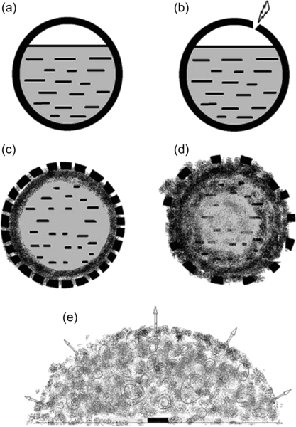
Figure 4.21 The simulation sequence of the instantaneous two-phase release, starting from (a) the initial condition; (b–d) the evolution of the release; and (e) the complete release resulting in the total integration of the flask. Reproduced by permission with Tan et al. (2011).
• The building structures could have a significant impact on the fireball evolution, as the local turbulence caused by interactions between the fluid with obstacles and corners may result in “hot spots.”
• In the early phase (the initial phase), the fireball is cool, rich in fuel, and lean in oxygen. The highest temperature was only reached after the fireball had risen above the facility corresponding to the uplift phase.
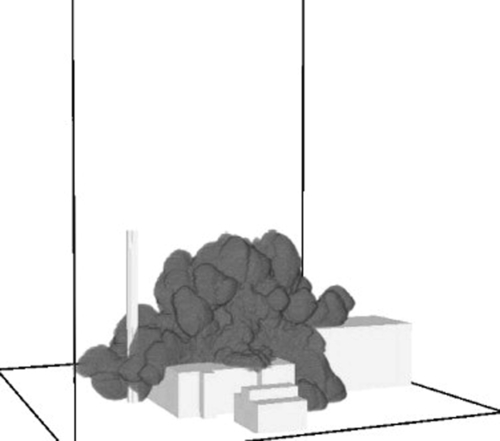
Figure 4.22 Graphical rendering of the fireball resulted from the impact of an airplane on a nuclear plant. Reproduced by permission with Luther and Muller (2009).
4.4.3. Deflagration to Detonation
Deflagration to detonation (DDT) is an important phenomenon in the context of process safety because of its devastating consequences. The nature of DDT and factors influencing DDT are currently subjects of ongoing research efforts. There are several theories to elucidate the mechanism behind a DDT phenomenon. For example, Sherman et al. (1989), by analyzing experimental data from the large-scale tests of hydrogen–air mixtures at the Sandia National Laboratory, proposed that DDT could occur when the shock fronts generated from the expanding unburned gas and those generated by the autoignition of preheat-unreacted mixture merge together (Sherman et al., 1989; Middha and Hansen, 2008). Other theories have been developed such as “local explosion” proposed by Oppenheim (Meyer et al., 1970), the “Shock Wave Amplification by Coherent Energy Release” (SWACER) concept proposed by Lee et al. (1978), or the instabilities caused by sudden venting by Dorofeev et al. (1995) and Middha and Hansen (2008). However, those theories have not been able to provide a full picture of what really happens or led to a practical mechanism behind the observations in DDT events in experimental works. Similarly, at this state, because of the complexity and the lack of clear understanding of DDT mechanisms, CFD modeling works on DDT only to try to shed light on the question of whether CFD as it is today is capable of describing DDT events. Current CFD studies on DDT could be divided into two different approaches: one is trying to precisely simulate a DDT event using available computational resources, and the other is trying to predict the possibility of DDT event in an indirect way.
The first approach is pursued by Oran's research group and other researchers efforts in simulating DDT from first principles have been published (Khokhlov and Oran, 1999; Khokhlov et al., 1999; Gamezo et al., 2001, 2005, 2008; Tegner and Sjogreen, 2002; Oran and Gamezo, 2007; Vaagsaether et al., 2007). An extensive list of several notable CFD simulation studies conducted to understand and predict DDT is also included in their review (Oran and Gamezo, 2007). The main objective of their current research is to provide an insight into DDT and to answer how, when, and where DDT occurs, mainly by numerically recreating and analyzing laboratory experiments. Even though their simulation systems were typically simple in a macroscopic view (i.e., shock-tube experiments), they pose formidable challenges because the simulation system has the capability to resolve up to 12 orders of magnitude ranging from the size of the system to the flame thickness (Oran and Gamezo, 2007). Through a series of sophisticated simulations, they have identified that shock–flame interactions play a central role in creating the environments leading to DDT. In these positive feedback interactions, the turbulent flames enhance the shock and vice versa, generating conditions leading to the formation of “hot spots,” or the ignition center of unreacted fuel mixtures that ultimately produce a detonation. They also have shown, through their simulation results, that the obstacles and boundary layers are critical in creating the suitable conditions for “hot spots” formation.
Even though these efforts could ultimately bring forward better understanding of the nature of DDT, the current computing resources only allows CFD simulation to be conducted in relatively small 2D or 3D systems; thus, predicting the possibility of DDT in realistic large-scale geometries such as offshore platforms or refineries by conducting first-principle CFD simulations may not be possible in the near future.
In the latter effort, notably works from Gexcon with their FLACS simulation packages, instead of directly simulating DDT, their efforts are on evaluating the likelihood of a DDT event (e.g., identifying whether DDT is likely in a given scenario and indicating the regions where it might occur) (Middha and Hansen, 2008). They proposed using a key indicator such as a parameter proportional to the spatial pressure gradient across the flame front or the normalized spatial pressure gradient (Middha and Hansen, 2008). This parameter provides visualized information on when the flame front captures the pressure front, which is the case in situations when fast deflagrations transition to detonation. Reasonable agreement was obtained with experimental observations in terms of explosion pressures, transition times, and flame speeds. By calculating this indicator for a given system, the likelihood of DDT could be inferred. For instance, Middha and Hansen (2008) proposed that the magnitude of this indicator around 10 or larger indicate a high possibility of DDT. The normalized spatial pressure gradient is calculated from the following equation (Middha and Hansen, 2008):
![]() (4.18)
(4.18)
where P0 is the initial pressure, and Xcv is the grid resolution.
A newer model has been introduced by GexCon to take into account the comparison of detonation cell size with geometrical dimensions, thus, correcting some of the short comings of CFD predictions by using the normalized spatial pressure gradient indicators such as DDT occurrence in very small geometries in which a detonation front may not be possible to propagate or in regions where there is insufficient fuel. The new indicator is introduced as DDT Length Scale, or DDTLS, which is calculated from the relevant geometric length in FLACS, the LSLIM:
![]() (4.19)
(4.19)
where DDTLS is a key parameter to predict the occurrence of DDT, LSLIM is the relevant geometric length scale in FLACS, and λ is the detonation cell size.
Figure 4.23 shows a result from a 2D CFD simulation in which the DDTLS is presented for a detonation tube experiment at two different times. According to GexCon, this new model has been shown to be able to predict with reasonable accuracy in multiple validation experiments. For example, in a detonation experiment using three detonation tubes with diameters D at 5, 15, and 30 cm at McGill University, the new model predicted that the DDT is most likely to occur near the baffle of the 30-cm tubes (DDTLS is around 20), while the possibility of having DDT in a smaller tube is lower (DDTLS is around four for the 5-cm tube). In other validation tests such as the GexCon 1.44 m explosion channel tests, or the Fh-ICT lane experiments, the tests conducted by SRI International and tests in the EU-sponsored HYCOM project, the simulation results were in reasonable agreement with the experimental data.

Figure 4.23 Graphical representation of the DDT length scale (DDTLS) results in the 30 cm diameter detonation tube. The top is the CFD simulation result at 14 ms and the bottom is at 17 ms. Reproduced by permission with Middha and Hansen (2008).
This new model is still in the development stage, and multiple challenges still need to be solved before it can be applied in industry for DDT prediction. For example, the relevant geometric length scale in FLACS (LSLIM) is an important parameter to obtain the DDTLS, but it is not clear how GexCon calculates this parameter in different scenarios, particularly because FLACS uses the Cartesian/PD approach to present the geometry. Further, the detonation cell, λ, is currently calculated using a fitting equation against available experimental data; this kind of fitting equation, as noted by Middha and Hansen (2008), is only valid within the range of the experimental data and may not be available for all kinds of fuel. Nevertheless, the results show some promise in its capability to predict the likelihood of DDT, and with further development it could be a very useful tool in process safety.
4.4.4. Dust Explosion
Complete understanding and a full description of dust explosion using CFD are still a formidable question in process safety. There are several challenges associated with dust explosion simulation using CFD, namely (1) complex computational domain involving internal geometries at industrial scale; (2) complex transient, turbulent, compressible two-phase flow (solid or particle and gaseous); and (3) complex incomplete combustion model involving rapid phase transitions (solid phase to gas phase) and multiple chemical reactions (Skjold, 2010). Unlike other types of CFD simulation such as dispersion or VCE, the first challenges, complex geometry representation involving internal system at an industrial scale, happens to be the most straightforward obstacle in CFD dust explosion simulation, while for the other two, there is need for better mathematical models describing the turbulent flow of dust clouds, models describing the combustion associated with combustible dust particles to accurately simulate dust explosion. Because of the chaotic and random nature of a combustible dust cloud, the inconsistency of available experimental data, even with data from standardized methods such as 20-liter vessel dust explosion experiments, adds more obstacles to the efforts of establishing a reliable CFD methodology for effective prediction of dust explosion hazards (Skjold, 2007).
Several key factors involving the dust cloud explosion listed by Eckhoff in his book Dust Explosion in Process Industries are (Eckhoff, 2003):
• Chemical composition of the dust, including its moisture content.
• Chemical composition and initial pressure and temperature of the gas phase.
• Distribution of particle size and shape in the dust: this distribution determines the specific surface area of the dust in the fully dispersed state.
• Distribution of dust concentration in an actual cloud.
• Distribution of initial turbulence in an actual cloud.
• Possibility of generation of explosion-induced turbulence in the still unburned part of the cloud (location of ignition source is an important parameter).
• Possibility of flame front distortion by mechanisms other than turbulence.
• Possibility of significant radiative heat transfer (highly dependent on flame temperature, which in turn depends on particle chemistry).
Therefore, the capability of an ideal CFD model should be sufficient to describe all those factors in order to accurately predict the characteristics of a dust explosion phenomenon. However, with current computing power, certain simplifications must be devised so that CFD simulation is feasible for dust cloud explosion.
4.4.4.1. Turbulence model
Modeling accuracy of a particle-laden turbulent flow in dust explosion simulation is a formidable challenge for many reasons. For example, dust particles, because of their wide distribution in size, density, and shape, never form a perfect, uniform dispersed cloud. This complexity, in CFD simulation, generally, is solved by certain simplifications such as uniform particle size distribution or noninteraction between particle assumptions. In this way, dust–air flow variables can be cataloged into two classes based on multiphase submodels: (1) Eulerian–Eulerian (E–E) model considers particle phase as a fluid phase; and (2) Eulerian–Lagrangian (E–L) model in which the particles are treated as a noncontinuous discrete phase (Zhong and Deng, 2000; Radandt et al., 2001; Zhong et al., 2001; Skjold et al., 2005; Zhang and Chen, 2007).
In the E–E model, the dust particles and air are assumed to be in thermodynamic equilibrium or, more specifically, they have the same velocity and temperature, implying that the size of particles are relatively small with uniform temperature throughout the particles (Skjold, 2007; Shi et al., 2009). Dust particles are further assumed to not contribute to the pressure of the system, and dust–gas mixtures behave like ideal gas. This assumption is reasonable when the size of the dust particle is relatively small, the density of the cloud is low and the thickness of the actual combustion front is much smaller than the characteristic dimension of the problem under consideration.
The second model, the E–L model, presents a more realistic system in which dust particles are treated as separate discrete phases, or the Lagrangian phase. This model allows simulated dust clouds to have different sizes, velocities, and interactions between particles, thus avoiding the thermodynamic equilibrium assumption used in the E–E model. The flow and combustion properties of dust particles (i.e., trajectories, mass changes, motions, and combustion) are calculated in Lagrangian coordinates (Radandt et al., 2001). However, the E–L approach requires much more computing power than the E–E model, indicating that it may not be applicable for large-scale simulations of dust explosions in the near future.
4.4.4.2. Combustion models
The combustion model used in dust explosion simulation is to describe the rate of the combustion process of premixed dust clouds (e.g., rate of conversion from reactant to product) and to define the reaction zone (Skjold, 2007). The combustion process for dust particles is much more complicated to be modeled in comparison to those of gaseous mixtures because of several issues involved such as multiple-step process, incomplete reactions, and complex product formation. To address this issue, Krause and Kasch (2000) divided and categorized the whole combustion process into a number of successive and manageable steps, including (1) devolatilization of the volatile fraction of the solid fuel, (2) mixing of the volatiles with oxygen in the gas phase, (3) combustion of the volatiles, and (4) combustion of the remaining solid fraction, which consists of mostly char. Further simplification is often applied to reduce this multiple-step complex process into solvable combustion problem in modeling. For instance, Collecutt et al. (2009) used the assumption that only CH4 and H2 were extracted from volatile, thus using single-rate Arrhenius equations to model two gas phase combustion reactions:
CH4 + 2O2 → CO2 + 2H2O
2H2 + O2 → 2H2O
and a reaction on the surface of the char particles:
C + O2 → CO2
This combustion model was used in a 3D CFD model using OpenFOAM, an open source CFD code, to study coal dust explosions and their suppression in underground coal mines (Collecutt et al., 2009). This study is part of a larger funded project to develop a practical active explosion barrier, specifically to develop the specifications for a prototype active explosion barrier which was designed as a ring of water injectors at the end of the tunnel. The simulation results so far were validated against a range of explosion conditions in the Simtars Siwek 20-L chamber and the 200-m explosion tunnel.
4.4.4.3. Published CFD studies in dust explosion
CFD modeling studies published in the literature could be divided into two groups based on the used aforementioned multiphase approaches: E–E or E–L approach. The former has been used in more CFD simulation studies because it is less expensive in terms of computing resources compared to the latter (Radandt et al., 2001; Zalosh, 2008). For example, Krause and Kasch (2000) developed a CFD model for vented dust explosion simulations using an FLUENT commercial CFD package to simulate and analyze time-dependent 2D or 3D local distributions of flow velocities, density, pressure, enthalpy, and species concentrations. In this model, the two-equation k–ε turbulence model with wall and buoyancy correction was used. They used an Arrhenius combustion reaction rate for laminar flames, and a Magnussen-Hjertager model for turbulent flames, and a multiple-step solid phase reaction model including devolatilization, gas phase mixing, and combustion and char combustion. This CFD model was used to calculate the laminar flame propagation through a mixture of lycopodium powder with air in a vertical tube of 2 m in length and 100 mm in diameter. An assumption in which the tested system was a time-dependent 2D laminar flow, particles with negligible inertia, and ignition near the closed end was used. It was further assumed that during devolatilization, mainly propane is released at an amount equivalent to the volatile content of the solid and combusted in the gas phase for further simplification of the combustion model. This simulation had good agreement with the experimentally observed flame speed, which subsequently was used to calculate dust concentration distributions in a 40-m3 silo, focusing on the flow and turbulence fields and the particle distribution. The results from this CFD model can be used for tests in which dust concentration and turbulence parameters have not been measured. It is also useful to predict the homogeneity of a dust cloud in real size, complex geometries, helping establish operating conditions to avoid the formation of dust clouds in the “optimum” range of concentration.
GexCon also applied the E–E approach in their effort to develop a CFD code called Dust Explosion Simulation Code (DESC) in order to simulate dust explosions in large-scale complex industrial facilities (Skjold et al., 2005, 2006; Skjold, 2007; Shi et al., 2009). DESC is part of a larger combinatorial project that uses both modeling and experiments to achieve a more comprehensive understanding and obtain more and better data on important but relatively not well-known aspects of dust explosion such as dust lifting and dust cloud formation. A review of the DESC project including summaries of the various sub-projects has been published (Skjold, 2007). The modeling parts in the DESC project include (1) the development of a combustion model for the turbulent dust cloud and (2) the development and validation of a CFD code. The sub-projects of the DESC include:
1. Turbulent flow measurement to measure the decay of the dispersion induced and to extract the empirical decay formulas for the root mean square of the turbulent velocity fluctuation and the integral turbulent length scale;
2. Measurements of burning velocities and flame speed to obtain the empirical correlation between the laminar and turbulent burning velocities, or the flame propagation velocity relative to the unreacted mixture under laminar and turbulent flow conditions; and
3. Dust dispersion phenomena to understand the mechanisms of the dust cloud formation (e.g., the process of lifting dust layers into dust suspensions) (Zydak and Klemens, 2007).
DESC CFD simulation code is based on the commercial FLACS CFD code developed by GexCon. The geometry is presented by the Cartesian/PDR model, turbulence by the two-equation k–ε model and particle-laden flows by the E–E multiphase approach. The particle-air mixture is assumed as an equilibrium mixture in which the dust particles are in dynamic and thermal equilibrium with the gaseous phase. The turbulent burning velocity is calculated by using the following equation:
![]() (4.20)
(4.20)
where SL is the laminar burning velocity of the dust cloud, St is the turbulent burning velocity of the dust cloud,  is the root mean square of the turbulent velocity fluctuation, and lI is the integral turbulent length scale.
The DESC dust explosion CFD code has been validated against several dust explosion experiments described in literature (Skjold et al., 2005, 2006) and has achieved reasonable agreement between the prediction results and the experimental data. DESC has been used to estimate the flow conditions inside the roller mill during normal operating conditions (van Wingerden et al., 2011) and in a filter system (Shi et al., 2009).
Large-scale comparisons to evaluate the effectiveness of DESC models also have been conducted. For example, DESC has been used to simulate large-scale explosions in 20- and 2-m3 interconnected cylindrical vessels designed by the UK Health and Safety Laboratory (see Figure 4.24). In this test, four different types of dusts including coal, silicon, and two types of potato starch were used as the representative of a wide range of combustible dust materials. One of the notable conclusions from this experiment is that there is poor repeatability of the experimental data, even between identical test settings, posing a significant challenge to validate the CFD model. Ideally, the necessary data to validate the CFD model would consist of relevant turbulence parameters, dust concentration, flame temperatures, burning velocity, and flow velocity, etc. In practice, it is not easy to obtain those data because of several reasons such as the reliability of the measuring method or the repeatability of the large-scale testing. Currently, only a beta version of the code, the DESC version 1.0 released in 2005, is available. Further development and validation are needed before DESC could be used as a full-fledged dust explosion predictive tool.

Figure 4.24 Rendering of the simulation system and the results using DESC. The top figure presents the simulated system and the bottom figure presents the simulation results of the dust explosion. Reproduced by permission with Skjold (2007).
The E–L approach, due to its higher cost of computing power, has a limited number of CFD simulation studies reported. Radandt et al. (2001) used the E–L model to conduct 2D CFD simulation for dust explosion in a closed vessel system with different height/diameter ratios. This CFD model used both gas phase and heterogeneous surface combustion of solid particles and took into account the heat loss to the vessel walls. In this model, the two-equation k–ε turbulence model was used for the turbulent flow. This modeling setup achieved good predictions for dust explosions in vessels with varying height/diameter ratios and agreed with experimental data. Although the calculations were limited only to 2D simulations, it can be seen that a similar approach can be extended to a 3D model for a realistic prediction at the industrial scale.
Zhong and Deng (2000) also applied similar E–L approaches in their CFD modeling of maize starch explosions in a large industrial-scale 12-m3 silo. The initial conditions including dust concentration, flow velocity, and turbulent RMS velocity in the silo in their CFD simulation were obtained from published experimental data. In their simulation, they took into account more factors known to have significant effects on the dust dispersion and combustion, including “dust granule” to consider dispersion efficiency, vaporization of water from particles, and radiation in the gas phase and between the gas/particle phases. The two-equation k–ε turbulence model was used to model turbulent flow. For volatile combustion, the eddy break-up model was used with the assumption that only CH4 and CO were extracted from volatile, and CO was generated by surface reaction of solid carbon. The combustion process was modeled as two completely irreversible reactions:
2CO + O2 → 2CO2
CH4 + 2O2 → CO2 + H2O
Although this simulation result has not been compared with experimental data, this promising result suggests that this model could be developed into large-scale realistic 3D geometry simulations of dust explosions with better particle motion and combustion models so that it can be applied in the design process.
..................Content has been hidden....................
You can't read the all page of ebook, please click here login for view all page.