Search in book...
Toggle Font Controls
Create new playlist

Name your new playlist

Playlist description (optional)
Sign In

Email address

Password

Forgot Password?

or

Continue with Facebook

Continue with Google
Sign Up

Full Name

Email address

Confirm Email Address

Password

or

Continue with Facebook

Continue with Google

Chapter 3

Molecular-Level Modeling and Simulation in Process Safety

Abstract

Molecular modeling is the science (or art) of representing molecular structures numerically and simulating their behavior with the equations of quantum and classical physics. Investigating chemical and material problems at an atomistic scale through capturing and understanding molecular interactions requires effective implementation of molecular modeling or computational chemistry techniques. Enabling ourselves to perform modeling at the molecular level empowers us with the ability to dig deeper into the characteristics of hazardous chemicals and processes, which are otherwise difficult and expensive to get through experimental observations. Application of molecular modeling has significantly increased in recent years and among others has been used in design and development of novel materials, drug discovery, protein engineering, microelectronics, and hydrogen storage. In here, we demonstrate how we can benefit from proven molecular modeling techniques for addressing process safety concerns.

Keywords

Ab initio; Aerosol; Carbon nanotube; Density functional theory (DFT); Dust explosion; First principles; Flammability; Flash point; Graphene; LFL; Molecular dynamics (MD); Nanotoxicity; QNTR; QSAR; QSPR; Quantum mechanics; Reactive hazards; Thermal runaway reaction; UFL; Water reactive chemicals

3.1. Introduction

Life … is a relationship between molecules.

Linus Pauling (Hager, 1995)

Molecular modeling is the science (or art) of representing molecular structures numerically and simulating their behavior with the equations of quantum and classical physics (Frenkel and Smit, 2002). Investigating chemical and material problems at an atomistic scale through capturing and understanding molecular interactions requires effective implementation of molecular modeling or computational chemistry techniques. The terms (“molecular modeling” and “computational chemistry”) are collectively used to refer to the theoretical methods and computational techniques used to model or mimic the behavior of molecules. It is a branch of chemistry which implements computer simulation of atoms and electrons to assist solving chemical and material problems. Simply put, it is a merger of:

• Physics of a system at the atomistic level

• Mathematical representation of the same in a solvable form

• Set of computational algorithms for solving the developed set of differential algebraic equations.

The type of problems that can be addressed through implementation of computational chemistry tools and techniques can be broadly categorized into (Lewars, 2010):

• Optimization of molecular geometry

• Energetics of molecules and transition states

• Chemical reactivity

• Infrared (IR), ultraviolet (UV), and nuclear magnetic resonance (NMR) spectra

• Molecular interactions

• Physical properties of a molecule

Molecular modeling empowers us with the ability to dig deeper into the characteristics of hazardous chemicals and processes, which are otherwise difficult and expensive to obtain through experimental observations. Application of molecular modeling has significantly increased in recent years and, among others, has been used in the design and development of novel materials, drug discovery, protein engineering, microelectronics, and hydrogen storage. While it has the potential to replace unnecessary experiments, insight gained from it can guide a new set of experiments. The realized potential of molecular modeling among researchers is illustrated through Figure 3.1. The figure is constructed based on a search in ISI Web of Science for citation record of highly cited English-language papers implementing molecular modeling studies within the engineering domain.¹ The trend of increasing citations, as illustrated in the figure, testifies to the increased utilization of molecular modeling tools and techniques for engineering studies.

For our purposes, within the realms of molecular modeling, the set of molecular modeling approaches can be broadly categorized in the following way, each of which can be implemented based on the problem objective:

1. Quantum mechanics/ab initio

2. Molecular mechanics

3. Molecular dynamics and Monte Carlo

4. Quantitative structure–property relationship (QSPR)/quantitative structure–activity relationship (QSAR)

The flow of this section starts with a brief introduction of the computational chemistry techniques, followed by application of the approaches for addressing problems related to industrial process safety. Figure 3.2 demonstrates some of the approaches used in modeling and simulation of materials at the molecular level.

Before digging deeper into the application of molecular modeling approaches, one needs to think about:

• Suitable methods for addressing the problem objective

• Suitable and accessible software for the purpose

• The availability of potential or force field parameters for molecular dynamics simulations

• Tradeoff between available computational resources and system size to be studied

Table 3.1 illustrates the computational cost associated with various levels of molecular modeling approaches. While solving Schrödinger's equation is never an option, choice of the remaining three depends on the answers to the concerns just specified.

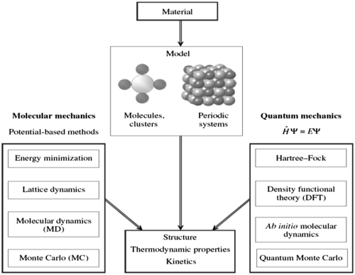
Figure 3.2 Various computational techniques used for modeling and simulation of materials at the atomistic scale (Stølen and Grande, 2004).

Table 3.1

Various Computational Methods and Their Scaling With System Size (Lee, 2011)

Methods	Scaling	N_max (atoms)
Schrödinger	O(e^N)	1
Hartree–Fock	O(N⁴)	∼50
DFT	O(N) ∼ O(N³)	∼200
Molecular dynamics	O(N)	10^7–11

3.1.1. Quantum Mechanics/Ab Initio approaches

The rules of application of quantum mechanics are unquestioned and the accuracy and precision of its predictions are unsurpassed in the entire history of science. Although heated debate continues about how quantum theory should be interpreted, there can be no debate about whether the theory is fundamentally correct (Baggott, 2011).

Quantum mechanical calculations are fundamental in nature and deals with physical phenomena at the atomistic scale where the units are in the order of Plank's constant (6.62606957 × 10⁻³⁴ m² kg/s). Two equivalent formulations of quantum mechanics were derived by Schrödinger and Heisenberg. The Heisenberg approach (Heisenberg, 1925) came from formulation of the quantum theory through development of matrix mechanics while working on calculating the spectral lines of hydrogen. The other formation, which later became the basis for nearly all computational chemistry methods (Young, 2004), is Schrödinger's wave formulation (Schrodinger, 1926) of quantum mechanics.

His methods were rapidly adopted by other investigators and applied with such success that there is hardly a field of physics or chemistry that has remained untouched by Schrödinge's work (Pauling and Wilson, 1985).

The starting point of Schrödinger's wave formulation equation was the well-known classical wave motion equation that interrelates the space and time dependencies of any waveform through a wave function, generally represented as

ψ

$ψ$

(psi). It is also known as probability amplitude functions. Schrödinger introduced mathematical description of electron as a wave for enabling the wave equation to provide meaningful solutions. The equation is represented as

$\hat{H} ψ = E ψ$ $\hat{H} ψ = E ψ$

where

\hat{H}

$\hat{H}$

is the Hamiltonian operator,

ψ

$ψ$

is the wave function, and E is the energy. It represents the quantum version of the traditional Hamiltonian equation and stands for the total energy of particles exhibiting wave properties. This means that the differential operator, for the total energy of a system, the Hamiltonian operator, operates on the wave function to yield the total energy of the system. The name of the equation has been given as wave equation as it is a second order differential equation with respect to the coordinates of the system, somewhat similar to the wave equation of classical theory. However, the similarity is not close (Pauling and Wilson, 1985).

The wave function

ψ

$ψ$

, is a function of the electron and nuclear positions. The significance of a wave function is that the square of a wave function represents the probability of finding an electron per unit volume. Hence, the wave function is a fundamental system property of a molecule and is the central entity in all quantum mechanical calculations. In order to obtain a physically relevant solution of the Schrödinger's equation, the wave function must be continuous, single-valued, normalizable, and antisymmetric with respect to the interchange of electrons (Young, 2004). Theoretically, the mathematical foundation of quantum mechanics is precise enough to ensure exact estimation of molecular properties. However, in practice, the exact solution has been obtained for only one-electron systems. In lieu of that, a plethora of methods have been developed over the years for finding approximate solutions of Schrödinger's representation of multiple-electron systems.

The various methods in quantum chemical calculations refer to the different types of approximation of the solution of Schrödinger's wave formulation equation for it to be effective for multiple-electron system. Finding and describing approximate solutions of electronic Schrödinger's wave formulation equation have been major preoccupation of quantum chemists since the very beginning of quantum mechanics (Szabo and Ostlund, 2012).

Currently, there are two main branches of electronic structure approaches used by researchers with various degrees of assumptions. While statistical errors, as realized in various experimental measurements, are not present in quantum chemical calculations, inherent errors appear and are associated with the various degrees of assumptions required to facilitate computational calculations. Based on the problem complexity, the practical approach to electronic structure calculations involves approximation, and it is vital to understand these along with its effects on the solution. The wave function–based methods start with Hartree–Fock (HF) method, in which many body wave functions are approximated as combinations of single-particle wave functions. Density functional theory (DFT), on the contrary, uses charge density of the system as an alternative representation to the many-body wave function. Since most calculations work on differences in energy (between two states) of systems, the accuracy of calculations is increased by error cancellation, as absolute errors in individual calculations owing to approximations nullify each other while estimating differences.

The HF method captures most of the important interactions involved in a system but does not incorporate correlation energy accounting for electron–electron interaction. It is reasonably good for computing the structures and vibrational frequencies of stable molecules and some transition states, but it is insufficient for accurate modeling of the energetics of reactions and bond dissociation. Accordingly, the HF method is used as a starting point for first principle calculations. Perturbation theories such as Møller–Plesset (MPn where n is 2 for the simplest level of theory) have been developed to go beyond the HF level of accuracy by providing perturbative corrections to HF results. The computational cost of MPn theories increase with values of n and is typically not used beyond MP5 (Foresman and Frisch, 1996). However, one must note that MPn theories cannot succeed where HF theory fails (Brazdova and Bowler, 2013). A comparison of different models in terms of accuracy and cost involved is presented in Figure 3.3.

In general, the relative accuracy of ab initio results can be presented as (Young, 2004):

$HF ≪ MP 2 < CISD ≅ MP 4 ≅ CCSD < CCSD (T) < CCSDT < Full CI$ $HF ≪ MP 2 < CISD ≅ MP 4 ≅ CCSD < CCSD (T) < CCSDT < Full CI$

DFT (Kohn and Sham, 1965) handles the difficulty of solving equations involving electron–electron equation by replacing the term through effective potential through mean field approximation. The theory computes electron correlation via general functionals (functions of functions) of the electron density. The first theorem of density functional theorem proves that the ground state energy from Schrödinger's equation is a unique functional of the electron density. This one-to-one mapping of ground-state wave function of a molecule to its ground-state electron density leading to the fact that by solving ground-state electron density of a molecular system allows one to estimate all molecular properties, including energetics and wave function. The second theorem on density functional theorem states that the electron density that minimizes the energy of the overall functional is the true electron density corresponding to the full solution of the Schrödinger's equation.

Figure 3.3 Comparison of various model performances in electronic structure calculations.

Despite the success of DFT, results from its calculation using LDA, in particular band gap calculation (difference in energy between highest occupied molecular orbital (HOMO) and lowest unoccupied molecular orbital (LUMO)) is inaccurate (Brazdova and Bowler, 2013). DFT approximates both exchange and correlation energy, while HF calculates exact exchange energy but ignores correlation energy. While hybrid functionals based on HF exchange energy rectify some of these deficiencies in DFT by adding a fraction of this exchange energy, the added component must be tested for the problem to be studied.

In quantum mechanics calculations, one needs to select a representation for wave function. This is done through specifying a basis set. This is analogous to specifying between cartesian or cylindrical coordinates for setting up a problem to represent position in space. Unfortunately, there is no perfect basis set, and a variety of basis sets are available to be chosen from. Ideally, in choosing a basis set, one must look for the following features (Brazdova and Bowler, 2013):

• Well adapted (i.e., few functions needed)

• Systematic convergence

• Good computational scaling with basis

Table 3.2

Description of Some Commonly Used Basis Sets in Electronic Structure Calculations

Basis Set	Description
STO-3G	Minimal basis, qualitative results—large systems
3-21G	More accurate results on large systems
6-31G(d)	Moderate set, common use for medium systems
6-31G(d,p)	Used where H is site is of interest, more accurate
6-31+G(d)	Used with anions, excited states, lone pairs, etc.
6-31+G(d,p)	Used with anions, excited states, lone pairs with H is site is of interest
6-311++G(d,p)	Good for final accurate energies but expensive

• Simple operations/calculations between basis functions

• Easy calculations of forces

• Bias free

Ideally, the basis set needs to be able to approximate the actual wave function sufficiently to give meaningful results. Table 3.2 provides description of some of the commonly used basis sets and their appropriate application domain.

Similar to any other computational approaches, electronic structure calculations require making some choices from a given set of models. Some generic recommendations are (Foresman and Frisch, 1996):

• Barring the computational cost, use B3LYP/6-31G(d) for geometries and zero point corrections and B3LYP with the largest practical basis set for energy calculations.

• For very large systems, performing multistage optimization such as performing HF optimization and frequency calculation followed by a B3LYP/6-31G(d) optimization may be more cost-effective.

• Somewhat in the similar lines of the above point, in cases where B3LYP/6-31G(d) is too expensive to perform, the best tradeoff is to use HF/3-21G(d) geometries and zero point corrections followed by the final B3LYP energy calculations.

• When AM1 geometries are practical for a molecular system, using B3LYP functional for the final single point calculation will still offer significantly more accurate results.

In general, to setup an ab initio or first principle–based calculations a researcher has to provide the following as an input:

• The molecular geometry (including spin state) and the system size

• Basis set and model selection for determination of the wave function

• Properties to be calculated

• Types of calculations and associated assumptions

These inputs can be provided in software GUI (Gaussian Inc.) or as explicit declarations inside input files (VASP).

3.1.2. QSPR/QSAR

In medicinal chemistry, regression modeling approaches at the molecular level, such as QSAR and QSPR, are exceedingly practiced. In varied studies, in a similar manner, attempts have been made to map the flammable activity of a molecule to its structural parameters (Gharagheizi, 2009). The QSPR takes the form of the following mathematical model:

$Activity = f (physiochemical properties and / or structural properties) + error$ $Activity = f (physiochemical properties and / or structural properties) + error$

The functional form is then found out through data mining of large data sets. Development of QSPR-based mathematical models to estimate flammability properties has gained popularity among researchers in recent times and is considered one of the modern flammability limits estimation methods. Structure–property (activity) relationships are qualitative or quantitative empirically defined relationships, between molecular structure and measurable properties or activities (Young, 2004). Expressed in a different way, QSPR and QSAR studies attempt to correlate several structural descriptors of a chemical compound with its physicochemical properties or biological activities. Ideally, to obtain a reliable and robust QSPR model, there should be an order of magnitude higher number of compounds than the number of parameters fitted (Young, 2004). The molecular descriptors are calculated to represent the molecular structure of the compound incorporating topological, charge, and geometric descriptor. Most of the molecular descriptors are easily determined, such as molecular weight, moment of inertia, and so on. The primary challenge in this approach lies in describing the molecular structure through appropriate molecular descriptor and selection of the appropriate modeling method (Yao et al., 2004). At present, molecular descriptors such as topological indices and quantum chemical parameters have been demonstrated to describe the structural property of a molecule (Karelson, 2000; Karelson and Lobanov, 1996; Todeschini and Consonni, 2008; Devillers and Balaban, 2000). Properties such as electronegativity, charge density, Fukui function, HOMO and LUMO energies, and electron affinity are examples of quantum chemical descriptors. A full set of list can be found in any book or book chapter on molecular descriptors (e.g., Todeschini and Consonni, 2008; Young, 2004). Since molecular descriptors are related to molecular structures, LFL values have also been estimated (Pan et al., 2009) using QSPR for organic compounds, where the estimation was carried out using the web-based DRAGON software program (Todeschini et al., 2006; Todeschini and Consonni, 2008, 2009; Tetko, 2003). The software, which has the capability of providing close to 5000 molecular descriptors, takes in molecular structure of a chemical as an input to calculate its molecular descriptors. As part of the process, which is briefed here next, the authors (Pan et al., 2009) optimized the geometry of all the molecular structures to obtain minimum energy configuration. The work used AM1 semiempirical quantum mechanics method and MM+ molecular mechanics force field in order to perform the geometry optimization through energy minimization of the molecular structure. But, based on accuracy requirement, minimum energy configuration can also be achieved by other quantum mechanical approaches such as the HF method or DFT.

Getting into the nitty gritty details of the QSAR or QSPR approaches is beyond the scope of this book. For the sake of clarity and convenience, we will briefly demonstrate the steps involved to develop QSPR or QSAR models for flammability properties. These are typically regression models that relate a set of predictor variables to a set of response variables. The underlying hypothesis behind a QSAR/QSPR model is that various physicochemical properties or biological activities of a compound are strongly coupled with its molecular structure. So once a reliable relationship has been established between a predictor and response variables, it can be used to predict the same properties for other compounds for which data do not exist. This is particularly helpful in designing novel materials but also of significant importance in regard to properties of existing chemicals. One may classify steps in developing QSPR-based approaches in several different ways. In the coarser side, only two broad segments (Pan et al., 2010) are defined:

1. Design and generate molecular descriptors

2. Constructing QSPR models with proper descriptors

A little more classification in the approach is presented (Yao et al., 2004):

1. Data collection

2. Molecular descriptor selection

3. Developing model correlation

4. Model evaluation and validation

An even better resolution set of key steps involved in the development of a generic QSPR/QSAR model can be shown as illustrated in Figure 3.4 (Knotts et al., 2001):

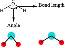
As one glances through the generic steps, one can see that accurate geometry optimization and deriving quantum chemical descriptors from that require detail-level modeling involving atoms and electrons. Since the values of many descriptors are related to the values of bond length and angles, having an optimized geometry of the chemical is required prior to performing any QSPR or QSAR calculations. This is where quantum mechanical or first principle–based calculations can be implemented to optimize its geometry by energy minimization techniques. If a suitable force field of the chemical of interest is available, molecular mechanics approach can also be implemented for geometry optimization of the molecule. The quantum mechanical approach is further used to generate the molecular descriptors from the optimized geometry and the obtained wave function. Once the geometry of the molecule is optimized, values of several descriptors are calculated using a suitable software. To select the best descriptors, first, descriptors with little or no variations across compounds are removed. By finding pairwise correlations between the remaining descriptors, only one among every two descriptors that are strongly correlated is retained so as to remove duplicate contributors and develop a more efficient model. To choose correlated descriptors, one has to define a high correlation coefficient (

ρ

$ρ$

) as the cut off point; for example, in the case of Pan et al. (2010), it was defined to be

ρ > 0.96

$ρ > 0.96$

. Examples of molecular descriptors can be atomic charges, dipole moment, HOMO and LUMO energies, etc. Considering the fact that the number of molecular descriptors typically can run into thousands, reducing the number of descriptors to the appropriate and most effective ones is an important step of the model development process. Through state-of-the-art hybrid approaches of coupling various regression analysis methods with genetic algorithm, such as that with multiple linear regression (Pan et al., 2010; Leardi et al., 1992) or partial least squares (PLS) regression (Leardi and González, 1998), optimal molecular descriptor set to represent mapping between the property set, such as flammability characteristics, and molecular descriptor set are identified. As a side note, in QSPR studies, chosing a appropriate regression technique for success of the model among choices such as multiple linear regression (MLR), PLS, and various types of artificial neural networks (ANN) is of prime importance (Pan et al., 2009). The final step in the development of the QSPR model is to validate the model through its predictive capability and robustness. Generally a good data set such as that from DIPPR 801, is divided into two sets for:

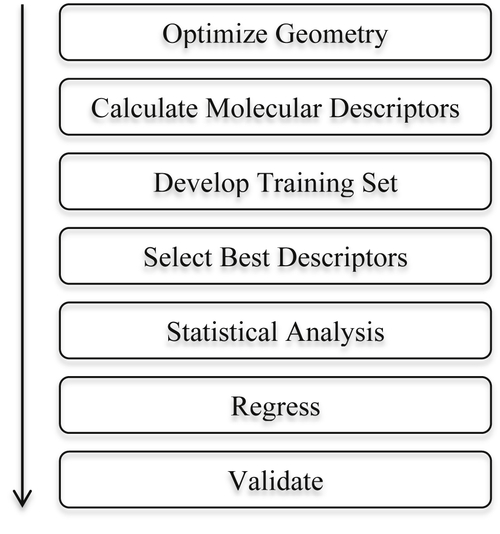
Figure 3.4 Typical steps in QSPR/QSAR in developing correlations. Reprinted with permission from Knotts et al. (2001).

1. Training and QSPR model development

2. Model validation

The steps involved in developing the QSPR model are very similar in nature to the development of other QSPR models as developed for process safety applications as demonstrated in earlier sections.

3.1.2.1. Data set

To develop QSPR-based mathematical models on predicting severity of dust explosibility, the initial step involves accumulating explosibility characteristics data, such as deflagration index (K_st) and maximum pressure (P_max), of dusts. This is a standard step in any QSPR method, where the first step is to gather quality experimental data for the properties or parameters to be modeled. In addition to the data of K_st and P_max, one also needs the data of the parameters whose function are K_st and P_max. Parameters correlated to K_st and P_max in dust explosion scenarios typically are representative particle size, moisture content, humidity, oxygen availability, shape, concentration, ignition source, and others. In general, the severity of dust explosion increases with smaller particle size. While an experimental data set is required to train and validate QSPR models, once built, it can be used to estimate dust explosion–related parameters for molecules of similar structures, eliminating the need for further experiments of chemicals whose structure–property relationship can be addressed by the developed QSPR models. In the work by Reyes et al. (2011), the authors used experimental combustion and explosion data of 31 chemical dusts from online database GESTIS-DUST-EX (Ifa, Gestis-Dust-Ex, 2014). The authors in their work used the median values for choosing the dust particle size. For the purpose of this study and validate their approach, the authors in this case extracted more data from other median values and created two specific data sets. One data set is to train and develop the molecular information–based mathematical model through the QSPR approach, and the other data set was used as a test set to validate their approach. It must be borne in mind that, based on the particle size distribution, median value of a data set may or may not be the best representation of the particle size to be used as an input for QSPR modeling. As an example, if the particle size is not uniformly distributed across the frequency diagram leading to large standard deviation, the calculation method for determination of representative particle size needs to be modified accordingly.

3.1.2.2. Geometry optimization

The QSPR methodology requires the incorporation of the structural information of the chemicals of interest. Since the aim is to build a mathematical model to map between the property of interest, explosivity characteristics in this case, and the chemical structure among others, for the purpose molecular modeling, optimization of the molecular structure yielding in its global minimum energy structure is of paramount importance. At the molecular level, the geometry can be optimized through implementing any of the following approaches, namely, first principle calculations, semiempirical quantum calculations, or implementation of classical force field methods using molecular dynamics as applicable to the chemical of interest. Owing to its fundamental nature, of the three methods, optimizing geometry of molecular structure using first principle calculations is expected to result in the most consistent and accurate results for any set of chemicals on interest, with a tradeoff with available computational resources as discussed in the introduction section of this chapter. In the particular study, by Reyes et al. (2011) the authors implemented DFT calculations at the B3LYP/6-31g level for optimizing the geometry of the molecules. The authors chose B3LYP function based on its effective performance for the systems involving organic compounds. A brief description along with pros and cons of various functionals in DFT methodology has been discussed at the beginning of this chapter.

3.1.2.3. Molecular descriptors

The optimized molecular structure obtained in the above step is used as an input to determine molecular descriptor. To generate these descriptors, various software packages are available. Typically, these packages derive a three-dimensional optimized molecular structure of the chemical of interest and calculate the descriptors using DFT. The initial substep within this step is to select a large number of descriptors and then reducing it to only the relevant ones and having only significantly sensitive descriptors with respect to the properties of interest. In general, the molecular descriptors can be of various kinds (Baatia et al., 2013), such as:

1. Constitutional (e.g., number of atoms and bonds)

2. Geometric (e.g., volume and surface area)

3. Topological (e.g., function of atom connectivity)

4. Electrostatic (e.g., partial charges)

5. Quantum chemistry derived (e.g., molecular orbital energies)

From this list, one can appreciate the importance of optimizing the geometry of the molecule prior to evaluate the molecular descriptor values. In the work by Reyes et al. (2011) the authors used the descriptors models and VAMP electrostatics in the simulation model of the Material Studio software package (Accelrys Materials Studio for Materials Modeling & Simulation, 2014). Starting with a set of 200 molecular descriptors, and following a heuristic method, the authors could narrow down their QSPR model to a set of 34 descriptors. Reduction of descriptors is necessary to increase the efficiency of the QSPR model and often done in steps. Further reduction in the number of descriptors can be done through various methods such as ability to calculate the descriptor for all structures, relevancy of the descriptor based on the property of interest, descriptors insignificantly sensitive to molecular structures and the like. In the work by Fayet et al. (2010b), the authors calculated 300 molecular descriptors using the CodessaPro software starting with the optimized molecular structure as obtained through DFT and AM1 calculations. Detailed definition of various quantum mechanical calculation–based and other molecular descriptors descriptors can be found (Karelson and Lobanov, 1996; Karelson, 2000).

3.1.2.4. Correlation-based model development

Depending on available data, its quality, and other factors, one can resort to several approaches in determining the correlations between the property of interest and the calculated molecular descriptors. For small data sets, a parametric space search technique such as GFA algorithm (genetic function approximation) can build several QSPR models from the available descriptors. In the study done by Reyes et al. (2011) application of the GFA technique resulted in two different QSPR models, each consisting of five parameters to estimate the K_st and P_max values.

3.1.3. Molecular Dynamics

First introduced by Alder and Wainwright (1957) by representing molecules as hard spheres, molecular dynamics has long been the tool for researchers to predict bulk properties and gain insight of various molecular systems based on atomistic scale calculations. In 1964, Rahman carried out the first simulation with Lennard-Jones potential on liquid argon as opposed to the hard sphere concept, which was being used until then. The need for molecular dynamics arose as, unlike ideal gases and metallic crystals, the properties of liquids were not easy to derive owing to their nonordered structure and nonideal behavior. Early models of liquids involved hard spheres and disks to represent molecules of a liquid system. Due to the same reason while molecular dynamics emerged as one of the main tool in predicting bulk properties of molecular systems, another method based on probabilistic approach called Monte Carlo, was also developed. Monte Carlo deals systems independent of time and hence is not capable of predicting dynamic properties. Metropolis et al. (1953) laid the foundation for modern Monte Carlo.

The theoretical basis for molecular dynamics modeling is statistical thermodynamics. Knowing the structure and dynamics of a system at the atomistic level can predict the bulk property of a system at the macroscopic level through application of statistical mechanics on the information obtained from molecular dynamics. Molecular dynamics simulation generates information of a system at the atomistic level indicating dynamic changes in a structure through estimating positions and velocities of all atoms of a system. According to classical mechanics, given initial position and velocity of a particle and the forces acting on it at any moment, one can predict its new position and velocity from Newton's second law of motion. The force on each atom at every time step is calculated by estimating the first derivative of the potential energy of the particle with respect to its position at that very instant. When more than one particle is involved in such a system, which is usually the case, different forms of interaction between them contributes to the potential energy. Identification and evaluation of various types of interactions between different types of particles are done with a set of rules called force field. A specific force field is developed based on information either obtained through experiments or first principle/ab initio calculations as introduced in the previous section. The practice in force field development involves development of force field for specific types of systems, such as biological or polymeric systems. Most types of interactions are all covered by a force field. In classical mechanics based calculations (molecular mechanics and molecular dynamics), the potential energy of a system is represented by analytical functions, namely the interaction force fields. The parameters of these functions are optimized so as to reproduce the fundamental properties, density, lattice parameters, vibrational frequencies, and the like. The functional forms are based on quantum mechanical arguments (Exp-6 form for van der Waals interactions, Morse form for bond stretch and harmonic form for angle bending, periodic-truncated Fourier series forms for torsion). Hence, a force field is the mathematical expression that describes the dependence of potential energy of a molecular system to that of the atomic positions of its constituent atoms. A force field has the ability to estimate the change in potential of a system from the knowledge of its initial condition of individual atoms, that is, atom positions and velocities along with the information on the perturbation of the system. The energy of a system can be written as

$E = E_{VAL} + E_{NB}$ $E = E_{VAL} + E_{NB}$

where

$E_{VAL} = E_{B} + E_{A} + E_{T} + E_{I}$ $E_{VAL} = E_{B} + E_{A} + E_{T} + E_{I}$

$E_{NB} = E_{VDW} + E_{C} + E_{HB}$ $E_{NB} = E_{VDW} + E_{C} + E_{HB}$

where E_B is energy due to bond stretching (two body); E_A is energy due to angle bending (three body); E_T is energy due to torsion (four body); E_I is energy due to out of plane configuration (four body); E_VDW is energy due to van der Waals interaction; E_C is energy due to columbic interaction; and E_HB is energy due to hydrogen bonding.

While the first four terms are attributed to bonded interactions, the last two terms are due to nonbonded interactions. The calculation of the nonbonded interaction is computationally expensive and contributes significantly to the overall simulation time. The electrostatic interactions are also called long-range interactions as they decay inversely with the value of “r” and hence contribute even for a large value of “r.”

Force fields are classified in different categories. There are second-generation force fields developed by high parameterization (e.g., CFF, PCFF COMPASS, etc.), rule-based force fields like Universal and Dreiding where parameters are decided by rules such as hybridization, classical or first-generation force fields like AMBER, CHARMM, and CVFFm which is based on parameterization but from experimental values as opposed to that of second generation, which is based on quantum input and special purpose force field.

Table 3.3 provides examples of functional forms as used in some of these force fields for estimating cost for departing from minimum energy configuration of a molecule.

In a molecular dynamics simulation, the system and its characteristics is defined by its structural behavior as captured by the force field within a given ensemble. The success of MD simulations is primarily due to the existence of statistical thermodynamics. It acts as the bridge between microscopic structure and the macroscopic bulk properties. One of the basic concepts in statistical mechanics is that if one waits long enough, the observer will be able to see almost all the microscopic states of the system for which the system will have the same set of macroscopic properties. This is termed as ergodicity. In other words, a set of macroscopic properties that completely defines a system has many microstates. These sets of macroscopic properties by which a system is defined completely are defined as different ensembles.

There are primarily four kinds of ensembles in statistical mechanics. Ensembles are nothing but a set of configurations (microstates) of the same set of molecules (making the system) while being consistent with the constraints with which the system is characterized macroscopically. The main four kinds of ensembles are namely microcanonical (N, V, E), canonical (N, V, T), grand canonical (T, V, μ), and isothermal–isobaric (N, P, T) ensembles where N stands for number of particles, V stands for volume of the system, P is pressure, T is temperature, and

μ

$μ$

is chemical potential. Different algorithms exist to ensure the constant property dynamics while running MD. All these ensembles are related to macroscopic property by the corresponding partition function.

Table 3.3

Illustration of Energy Forms in Bonded Interactions and Their Corresponding Functional Forms

Energy Forms		Example Functional Form(s)
Bond stretching		$\begin{matrix} E = \frac{1}{2} k_{e} {(R - R_{e})}^{2} \\ E = D_{e} {(e^{- α (R - R_{e})} - 1)}^{2} \end{matrix}$ $\begin{matrix} E = \frac{1}{2} k_{e} {(R - R_{e})}^{2} \\ E = D_{e} {(e^{- α (R - R_{e})} - 1)}^{2} \end{matrix}$
Angle bending		$\begin{matrix} E_{I J K} = \frac{1}{2} C_{I J K} {[\cos θ_{I J K} - \cos θ_{J}^{0}]}^{2} \\ E_{I J K} = \frac{1}{2} K_{I J K} {[θ_{I J K} - θ_{J}^{0}]}^{2} \end{matrix}$ $\begin{matrix} E_{I J K} = \frac{1}{2} C_{I J K} {[\cos θ_{I J K} - \cos θ_{J}^{0}]}^{2} \\ E_{I J K} = \frac{1}{2} K_{I J K} {[θ_{I J K} - θ_{J}^{0}]}^{2} \end{matrix}$
Torsion		$E_{I J K} = \frac{1}{2} V_{J K} {1 - \cos [n_{J K} (ϑ - ϑ_{J K}^{0}]}$ $E_{I J K} = \frac{1}{2} V_{J K} {1 - \cos [n_{J K} (ϑ - ϑ_{J K}^{0}]}$

• NVE or microcanonical: The value of macroscopic properties N, V, and E are constant in this ensemble. As these three macroscopic properties are kept constant, the values of pressure, temperature, and chemical potential are determined for the equilibrated system.

• NVT or canonical ensemble: The values of N, V, and T are constant in this ensemble.

• NPT or isothermal–isobaric ensemble: In this ensemble, as the name suggests, the different systems that are dealt with have the same values of N, P, and T.

• TV

μ

$μ$

or grandcanonical ensemble: Here, the values of T, V, and μ are kept constant. Any standard book (Sandler, 2010; Hill, 2012; McQuarrie, 2000) can be referred to for a detailed description of these ensembles and their relation to the macroscopic property of the material.

Sync Reading Stream

What's this?

..................Content has been hidden....................

You can't read the all page of ebook, please click here login for view all page.

Table of Contents for 3.1. Introduction

Create new playlist

Sign In

Sign Up