2.4. Present Approach to Process Safety
2.4.1. Risk and Hazard
“Hazard” and “risk” are often used interchangeably and treated as equivalent terms in informal communication. However, each term has its own distinct and precise usage in formal risk communication. A “hazard” is something with the potential to cause an undesired consequence by virtue of one or more of its inherent properties. Something with this potential is said to be “hazardous.” The severity of the consequences and the likelihood of those consequences are not addressed by “hazard.” The term “risk” is used to describe a measure of the probability of a consequence occurring and the severity of that consequence. Therefore, a “hazard” can be thought of as a potential source of harm and “risk” is a measure of the size of that potential harm (Modarres, 2006).
Hazards arise in a process and in life from a variety of sources including but not limited to (Crowl and Louvar, 2011):
• Objects or persons at elevation (potential for falls from a height)
• Toxic substances
• Flammable or explosive substances
• Substances stored under pressure
• Substances stored at extremes of hot or cold
• Conduction or build-up of electric charge
Two facilities can have identical hazards, possibly as a result of operating nearly identical processes, but have very different associated risk levels. Risk is traditionally defined as the product of the expected frequency and severity of a consequence (Crowl and Louvar, 2011):
![]() (2.88)
(2.88)
where f is the frequency of the event, usually expressed annually or monthly, and S is the severity of the consequence, usually expressed in monetary terms.
If barriers exist to prevent the consequence, the probability of these barriers succeeding or failing can be incorporated into the calculation of the event frequency.
 (2.89)
where IEF is the initiating event frequency, and PFDi is the probability of failure on demand of the ith barrier of n total barriers. If multiple hazards or consequences are possible, the total risk can be seen as the sum of the risks from the individual hazards and consequences (Modarres, 2006).
 (2.90)
Incidents and losses may be initiated by events or factors outside of system that may be beyond the control of the operators of the system. Similarly, losses may occur to the system or they may be caused by the system and inflicted on one or more recipients.
Risks are broadly grouped into five main categories: health, safety, security, financial, and environmental. Health risks principally involve disease and illness. Safety risks involve disasters, incidents, products, and technologies. Security risks pertain to war, terrorism, social unrest, crime, and misappropriation or misuse of information. Financial risks involve currency fluctuations, market fluctuations, interest rates, market share, bankruptcy, supply interruptions, and business interruptions. Finally, environmental risks involve contamination or damaging of the ecosystem (air, land, water, and space) with trash, toxins, noise, and odors (Modarres, 2006).
Risk analysis involves identifying, characterizing, managing, and disseminating information with regard to potential losses. Risk analysis, therefore, typically involves three elements or stages: risk assessment, risk management, and risk communication.
Risk assessment is the component traditionally thought of when risk analysis is referenced. It involves the estimation of event probabilities, frequencies of occurrence, and consequence severities. This assessment is normally handled by first identifying hazards, generating scenarios, identifying barriers where they exist, assessing the likelihood of the scenarios, and then estimating the consequences. A scenario deemed too unlikely to be credible may not warrant consequence analysis.
Risk management is principally concerned with managing uncertainties but is a highly complicated decision-making process. Resources are always limited, and it is infeasible for every hazard to be mitigated through the use of extremely expensive or complex systems. Additionally, it is impossible to reduce risk to zero. There will always be some residual risk that cannot be eliminated. As such, companies and management are required to define levels of acceptable risk. Once a risk is reduced to below this threshold value, further mitigation is unlikely as any additional resources are likely to be directed toward addressing other risks. If a risk has not been reduced to the level deemed acceptable but a further reduction of risk is cost prohibitive the risk can be considered conditionally acceptable (Modarres, 2006).
A risk can be referred to as being ALARP when it has been reduced to the point where further reductions in risk will cost more than they are expected to save through risk reduction.
Assessing risk also requires the expenditure of time and resources. A full, detailed, quantitative risk assessment will require more time and resources than a simple qualitative assessment. Management must decide how much effort to expend on assessing the risk from various hazards and scenarios. A hazard that is expected to produce low consequences is unlikely to be the subject of detailed analysis. A high consequence scenario, on the other hand, may warrant a thorough analysis.
Risk management is the most important part of risk analysis as only a proper allocation of resources will result in optimized risk levels and overall process safety.
Risk communication involves the dissemination of information with regard to the existence of risks, their likelihood and consequences, how the risks were identified and assessed, the assumptions and uncertainties involved in the analysis, and what steps are being taken or can be taken to manage the risks.
2.4.2. Methodology in Risk Assessment
Some major steps are common to all risk assessments. These include:
• Hazards identification
• Barrier identification
• Barrier performance assessment
• Exposure assessment
• Risk characterization
The methods for carrying out the assessment will vary depending on the type(s) of risk being assessed.
Hazards identification: The first step in the risk assessment process, as the name suggests, involves the identification of hazards, which result from all potential sources in the system. Some hazards are natural and some are artificially made. Some hazards are inherent to a material, or process. Some hazards are emergent, resulting or arising from a unique combination of materials, conditions, and circumstances. Once identified the hazards must be characterized in terms of their amount, intensity, and severity.
Barrier identification: Barriers are systems or structures that function as “obstacles [for] containing, removing, neutralizing, preventing, mitigating, controlling, or warning” of hazards (Modarres, 2006). Barriers can be active or passive. Passive barriers provide protection merely through their presence and do not require activation or the operation of some function to prevent or mitigate the hazard. Passive barriers include dikes, casings, natural circulation, and ventilation, among others. Active barriers require that they be activated or triggered to perform their function. Activation can be manual, through the action of an operator or other personnel, or automatic, usually triggered by some kind of sensor. Active barriers include cooling systems, alarms, automatic shutdown systems, drainage pumps, fire water systems, and foam fire suppression systems among others.
Barrier performance analysis: No barrier or protective system can be perfect. There will always be a chance that a particular barrier will fail when it is needed. An event that requires the action or the function of the system to avert a hazard is called a “demand” as it places a demand or a need to function on a system that normally sits and waits. The chance or the probability that the system will fail to function or function inadequately is known as the “probability of failure on demand,” or PFD. The PFD for a system can change over time because of age, degradation, damage, or overuse. Proper maintenance will slow down, but usually not prevent, this degradation.
The PFD for a system must be estimated through one of a variety of means, some of which are discussed in Yañes et al. (2002). There will always be uncertainties in the assessment of barrier performance and reliability. These uncertainties should be included in the final assessment and considered in the analysis.
Exposure assessment: This step attempts to predict the likely consequences of a barrier failure. If some or all of the barriers to a hazard fail, the effects of the hazard may be felt, either in full or to a lesser, mitigated degree.
Risk characterization: In the final step of the risk assessment, the magnitude of the consequences from various hazards and scenarios are estimated based on available information. These consequence estimates are combined with probability and frequency calculations to estimate the expected losses from each individual hazard and all identified hazards collectively.
The estimation of probabilities, frequencies, and consequences can be either quantitative or qualitative.
2.4.2.1. Nodes in risk assessment
Many of the risk assessment methodologies are involved and can be complicated. It is difficult, if not impossible, to apply many of them to an entire process from start to finish at the same time. It is therefore common, even necessary, to break up a process into sections, or “nodes.” A node generally consists of one major process vessel, often a reactor or a column, along with the associated process lines, instrumentation, and supporting equipment such as heat exchangers and settling tanks. Process can be divided into as many or as few nodes as necessary to facilitate the analysis. The analysis should, however, be able to consider how problems in one node might impact another.
2.4.2.2. Teams and information required for a risk assessment
All forms of risk assessment require extensive information about the process to be analyzed to be successful. The first step in almost any risk assessment is the collection of data and documentation on the process including detailed flow diagrams, instrumentation diagrams, chemical inventories, maintenance logs, and more. A thorough risk assessment will also require a diverse team that is knowledgeable with regard to the process and the likely outcomes or consequences of various abnormal events. Risk assessment teams should include leaders or facilitators, engineers, maintenance personnel, and operators.
2.4.3. Quantitative Risk Assessment
Quantitative risk analysis (QRA) attempts to estimate the probability or frequency of an event and its consequences. QRA seeks to arrive at a numerical value for the level of risk presented by a hazard. There will be uncertainty in these estimates that must also be characterized and quantified through established and accepted statistical means. An accurate QRA requires a large amount of data and information. In cases where data are sparse, quantitative analysis is difficult and uncertainties can be large. QRA also tends to be much more resource and time intensive than qualitative and semiquantitative approaches. Because of this, QRA is preferred in situations where the data, resources, and time are available in addition to justification with regard to the high risk and complexity of operations.
2.4.4. Scalability in Risk Assessment Methodologies
As a general rule of thumb, qualitative and semiquantitative approaches to risk assessment will scale better than quantitative methods. A true quantitative analysis is rigorous and computationally heavy. The complexity of the analysis will increase rapidly as the size and scope of the project increases. As a result, quantitative analysis is usually highly targeted and used to answer important questions with regard to scenarios of potentially high consequences.
Qualitative approaches tend to scale better between smaller and larger projects as the simplifying assumptions used in them prevents the calculations and data requirements from becoming overly burdensome.
2.4.5. Probability Based Approaches
Probabilistic risk assessment (PRA) is a procedure for examining the operation and interaction between parts of complex systems. A thorough PRA accounts not only for equipment but also for human elements, software, and control systems, all of which can fail. The PRA has the ability to identify the components that make the largest contributions to risk in the system. There are several steps to a PRA (Modarres, 2006).
1. Objectives and methodology definition
2. Information assembly and system familiarization
3. Identification of initiating events
4. Scenario development
5. Logic modeling
6. Failure data collection and performance assessment
7. Integration and quantification of risks
8. Uncertainty analysis
9. Sensitivity analysis
10. Risk ranking and importance analysis
11. Interpretation of results
Objectives and methodology definition: The scope and goal of the analysis as well as the expected final deliverables should be selected at the beginning of the analysis. Once the analysis is scoped and objectives set, a technique should be chosen from the options available, some of which are discussed here.
Information assembly and system familiarization: All the information needed for the analysis must be collected and then reviewed. Before beginning the analysis, all of the components of a system must be identified and understood.
Identification of initiating events: Generate a list of events that could set a hazardous event or consequence in motion. Functional block diagrams of the system may be helpful for this purpose. Initiating events should then also be grouped based on the required responses to the initiating events.
Scenario development: In principle, scenario development seeks to identify all possible pathways for the propagation of a hazardous event. This is not always possible or practical; however, there can be an infinite or nearly infinite number of scenarios depending on the system and hazard being analyzed. It is therefore sometimes necessary to select a representative set of scenarios that are thought to encompass most major or significant outcomes and consequences.
Logic modeling: Certain types of analyses, including fault trees and event trees, require the development of a logic model that models the dependencies of various systems on their base components.
Failure data collection and performance assessment: Estimation of failure rates and event frequencies will require data on the reliability and performance of all of the base components that make up the system. These data will need to be collected as an input to the calculations.
Integration and quantification of risks: The analysis is conducted and the final numerical outputs of the analysis are generated. Boolean reductions may be conducted at this time. Minimum cut sets should be identified, and the results of the analysis should be used to determine which components make the biggest contributions to risk in the system.
Uncertainty and sensitivity analysis: Uncertainty analysis will assess the expected margin for error in the final results based on the quality and quantity of the data and the assumptions used in the analysis. Sensitivity analysis examines the model and parameters used in the analysis as well as the assumptions used to conduct the analysis to determine the impact that each has on the final outcome. The analysis or model is said to be “sensitive to those parameters or assumptions that have the greatest impact on the results.” Sensitivity analysis and uncertainty analysis help focus attention and resources on those aspects of a PRA that might warrant further attention or consideration to improve the quality of the PRA.
Risk ranking and importance analysis: Components and systems should be ranked according to their importance to the system and its reliability. This can be done through a variety of means. Some importance measures are based purely on the mathematical contribution of that component to the overall risk of the system, while other methods rank components based on their contribution to the uncertainty of the analysis, called “uncertainty ranking.” Some methods rank the importance of a component by looking only at that component, while others rank the importance of a component based on its importance compared with other components and subsystems.
Interpretation of results: The interpretation of results is actually a continuous process in the PRA in which the outcomes of each stage of the analysis are examined and opportunities to improve the accuracy of the analysis are looked for. Interpretation of the results should continue until the analysis arrives at what is felt to be a reasonably stable and accurate input with acceptable uncertainties.
2.4.5.1. Fault tree analysis
Fault tree analysis seeks to determine how systems or hazard barriers can fail by starting with a highly specific top event or failure and work back to determine how that top level event could occur. As such, fault tree analysis is a deductive process in which the risk analysis team attempts to determine how an event might occur. Fault trees can be used to evaluate simple top level events for small systems or larger plants; however, fault trees for larger systems can easily grow to include thousands of events, spread out over hundreds of pages. Fault trees for simple events, like a tank overfilling, for example, can be constructed and evaluated in a few minutes if the required information is available. Large fault trees are frequently drawn and evaluated using computer programs.
The number of events that must be dealt with in a fault tree is controllable by limiting the resolution of the analysis. Nonbasic events can be left undeveloped in the analysis, especially if a detailed analysis of the event is not considered likely to be beneficial, in the interest of saving time or resources.
Fault trees are constructed from a variety of logic gates and event types. Some of most commonly used symbols in fault tree construction are shown in Figure 2.17.
There are several steps to developing a fault tree that can be expressed as:
1. Precisely define a top event.
2. Determine the conditions required for the top event.
3. Define the physical limits of the system and the scope of the analysis.
4. Determine which events will be considered nonallowed or too rare to be considered in the analysis.
5. Define the equipment configuration and the normal condition of the process.
6. Define the level of resolution, or how far the analysis will proceed.
7. Draw the tree, starting at the top and continuing until intermediate events have been explored and only basic events, external events, and undeveloped events remain.
8. Evaluate the tree, starting at the bottom with basic events, external events, and undeveloped events.
Drawing the tree can be conducted using the following sequence:
1. Select an event (top or intermediate).
2. Determine the conditions (events) required for this event and select appropriate gates (AND, OR, NAND, NOR).
3. Determine whether each condition is an intermediate event, basic even, external event, or undeveloped event.
4. Repeat steps one to three until all intermediate events are explored and developed. (Note: an event can be left undeveloped if it is not considered worth further exploration.)
The tree can be evaluated in the following ways:
1. Determine the failure probabilities of all basic, external, and undeveloped events.
2. Determine all minimal cut sets and/or success paths for the fault tree.
3. Calculate the probability of each cut set or success path to determine the probability of the top level event occurring.
or
2. Perform the necessary calculations across the logic gates associated with these events to determine the probability of the next level of intermediate events.
3. Repeat step 2 until the top level event is reached and its probability is calculated.
2.4.5.2. Event tree analysis
Event trees are most appropriate when the successful operation of the plant or a safety outcome to an emergency requires the chronological and independent operation of barriers and systems (Modarres, 2006). The sequential nature of the events becomes important in modeling the propagation of an incident and the role of various systems and barriers in determining the ultimate outcome (Crowl and Louvar, 2011). The event tree starts with what is appropriately named an initiating event and follows an inductive process to predict probable consequences (Modarres, 2006; Crowl and Louvar, 2011). The steps in an event tree analysis are typically thought of as (Crowl and Louvar, 2011):

Figure 2.17 Common fault tree symbols. Reproduced from Crowl and Louvar (2011).
1. Identify or select an initiating event.
2. Identify the systems that deal with or mitigate the initiating event.
3. Determine the order of the events.
4. Construct the event tree.
5. Determine the resulting event sequences and outcomes.
The event sequence and the sequence outcome are typically listed on the right side of the event tree. Trees are typically constructed with a successful (or positive) outcome taking the upper branch and a failure (or a negative outcome) taking the lower branch. Many event trees are constructed with two final outcomes: success and failure, safe and unsafe. However, because some barriers can act to mitigate or limit, rather than prevent, an incident, an event tree that includes such systems and barriers can be constructed with one or more intermediate outcomes. Branching of the tree does not always occur at every event for every pathway (Bahr, 1997). For example, two events in a sequence might be the operator manually shutting down the system and an automatic system shutdown in response to an alarm or trigger. The system can only be shut down once in the sequence. Therefore, if the operator is intended to take action first and successfully shuts the system down, then automatic shutdown will not function. The system is already in a shutdown state. The event tree for these two barriers would look like Figure 2.18.
Evaluation of event trees is handled using Boolean expressions to determine the probability of each outcome of the event tree.

There is no limit on the number of events/barriers that can be used or evaluated in an event tree analysis. The event tree can have as many branching events as are deemed necessary for the analysis. The technique is therefore infinitely scalable with regard to the complexity of the analysis.
The technique is also flexible. It can be applied to a wide range of systems and initiating events as it only requires the identification of a hazardous event and barriers designed to counter that event. This allows the method to be applied to tanks overfilling, reactors overheating, attacks on the facility, loss of outside power to part of the facility or the entire facility, and software glitches.
2.4.5.3. Bow-tie plots
A bow-tie plot can be looked at as a combination of a fault tree and an event tree. If the top level event of a fault tree is the same as the initiating event of an event tree, the plots can be arranged end-to-end and combined to form a bow-tie diagram. The bow-tie diagram is named because of the characteristic shape formed by it as the triangular shapes of the event tree and fault tree narrow to the process mishap in the middle as illustrated by Figure 2.19.
More generally, the bow-tie plot combines the deductive and inductive processes of the fault tree and event trees to allow a single diagram and analysis to trace a failure event from its root causes to its ultimate consequences. The bow-tie plot traces the path of a failure through the process control systems to the top level event and then through the protective layers of the mitigation system. The bow-tie plot traces from the basic failure events to the final outcome and consequences (Bahr, 1997). Because the bow-tie plot is a combination of a fault tree and an event tree, it enjoys the flexibility and scalability of the other two approaches.
2.4.5.4. Failure modes and effects analysis
Failure modes and effects analysis (FMEA) lists the ways (modes) in which components and elements in the system can fail. The likelihood and effects of each failure mode on the system are determined. Mitigating steps that can or should be taken are recommended based on the resulting scenario probabilities and consequences. FMEA is best applied to simple systems or systems with a limited number of parts or failure modes. It works well for simple systems and single pieces of equipment but it is not readily applicable to larger systems like whole processes and facilities.
The FMEA technique consists of a methodical study of component failures. Typically, this review starts with a diagram of the process that includes the most probable components that could fail and consequently create a safety hazard for the process. According to OSHA, the following list represents a typical FMEA and the process that should be used to perform this analysis.
• Potential mode of failure
• Consequence of the failure

• Effect on whole system
• Hazards class (qualitative)
• Probability of failure
• Detection methods
• Compensating provision/remarks.
• Recommendations
2.4.5.5. Bayesian networks
Thomas Bayes (1702–1761) developed the Bayes theorem, which facilitates the calculation of the probability of causes based on observation of effects. During the 1980s, the model was extended to relate the probabilistic relationships among statistically or causally related variables. Bayesian networks (BNs) were developed from probabilistic graphical structures designed to represent these relationships (Jordaan, 2005).
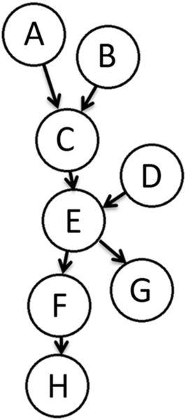
A BN is a graphical description of the direct dependencies among a set of variables. The directed graph is constructed with variable nodes and arcs connecting them. Each variable node has a node probability table or a conditional probability table of probabilities for each state of the node variable. There are “parent nodes” and “child nodes” encoded with the assumption that the value or state of the “parent node” variable influences the value or state of the “child node” variable. As a result, there must be no cycles back to a prior node in an arc on a graph to avoid circular reasoning. A “root” node has no parent nodes. It is the start of a chain and no other variables in the network influence it. A “leaf” node has no child nodes and therefore influences no other variables. In a directed chain of nodes, a node is an “ancestor” of another if it appears earlier in the chain and is a “descendant” of a node if it appears later in the chain. The set of parents of a node “X” is designated by Parents(X) or pas(X). All nodes that are not root or leaf nodes are “intermediate” nodes. The root nodes therefore represent original or initiating events and the leaf nodes are final effects or consequences (Jordaan, 2005; Fenton and Neil, 2012).
In Figure 2.20, nodes or variables labeled A, B, and D are root nodes. G and H are leaf nodes. A and B are parents of C, C and D are parents of E, which is a parent of F and G. F is a parent of H. The BN allows for us to take knowledge of the state of H to improve our knowledge of the state of F and to use knowledge with regard to the state of F and G to improve our knowledge E, working back through the chain. In the figure, C, E, and F are intermediate nodes. Nodes A, B, C, and D are ancestors of E, while F, G, and H are descendants of E.
BNs assume the Markov property is in effect. That is, the only dependencies that are in effect are the ones shown by the directed arcs and that unconnected nodes are conditionally independent.
When the state of a BN variable is observed or known, the “credibility” of the network changes and it must be conditioned by the new information. This conditioning process can be referred to as probability propagation, inference, or belief updating. Information flows in both directions, not just in the directions of the arcs. This results in different reasoning types in BN calculations: diagnostic, predictive, and intercausal. Diagnostic reasoning moves in the opposite direction of the arcs, it starts with effects and updates causes. Predictive reasoning moves in the direction of the arc and uses information on causes to update probabilities of effects. Intercausal reasoning involves effects with more than one cause. Observing the state of an effect with two or more causes increases the likelihood of all the causes; however, if the state of one cause is also known, the state of that cause can make the other cause(s) less likely. The other causes are therefore “explained away” (Korb and Nicholson, 2003; Jordaan, 2005).
Any nodes in a network can be “evidence” nodes, the state of which is known, or “query” nodes, the state of which is influenced by the evidence.
BN calculations are now normally handled by computer programs. But some of the calculations involved can be provided here. The probability of a set of values or states for all of the variables shown in Figure 2.20, P(A, B, C, D, E, F, G, H) can be given by (Jensen and Nielsen, 2009):
![]() (2.91)
(2.91)
However, because the Markov property is in effect, the probability of an event depends only on the state of events above it in a chain. Take the probability of C, P(C), as an example.
![]() (2.92)
(2.92)
As a further example, if we assume F and H are both variables with only two possible states, true or false, we can use knowledge of H to learn more about F. Say event H is the failure of a system to operate and event F is the failure of a component in that system, which can, but does not necessarily, cause the system to fail. Table 2.10 is the probability table for F, a component failure. Table 2.11 is the probability table for H, a system failure, given F (Fenton and Neil, 2012).
If we observe a system failure, we can update our estimate of the probability of the component failure, F. P(ε) is the marginal probability of the observed parameter:
 (2.93)
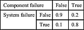
Given that the system failed, we can update the probability that the component has failed based on:
 (2.94)
Therefore, the observation that the system has failed increases the probability that the component has failed from 0.1 to 0.47.
As the prior example illustrates, BNs can be constructed to analyze systems of as little as two events, but they can also be used to analyze systems far more complicated than the system in Figure 2.20, with hundreds or thousands of events. Similarly to fault trees, once BNs exceed a certain size it becomes prohibitively difficult to construct the network and evaluate the system without the use of a computer; however, various computer programs have been developed for using BNs. Even with a computer, a large, complex network will be more time-consuming to construct. However, once the network is built, the availability of cheap computing power makes the method easy to use, even for relatively large systems.
2.4.6. Consequence-Based Approaches
There is an approach in risk analysis known as “consequence-only decision making.” In some cases the consequences of a scenario or situation are deemed to be so severe that a company or facility may decide to take additional steps to prevent or mitigate an event without determining the likelihood or expected frequency of the event. This is usually rare, but consequence estimation remains an important component in risk analysis.
2.4.6.1. Fire consequence modeling
A wide variety of models and equations have been developed over time to model various types of fires and predict the consequences thereof. An introduction to some of these models is presented in Section 2.1.4. Explosion consequence modeling is discussed in detail in Section 2.2.3. This section discusses some of the impacts and consequences of fires.
Impact on personnel
The primary danger to a person within the line-of-sight to a flame is thermal radiation, which will most often result in burns to exposed skin as well as the ignition or melting of clothing. Burns are classified in degrees, of which there are three, based on the depth of the burn, the extent of blistering, and the type of damage sustained. A first-degree burn is the least severe with only superficial burns, similar to most sunburns. A third-degree burn is the most severe with burns more than 2 mm deep, which affect nerve endings and cause a loss of sensation (Crowl and Louvar, 2011).
Skin will begin to burn at 45 °C (113 °F) and becomes nearly instantaneous at 72 °C (162 °F). Time to injury can be predicted for bare, unprotected skin using tables available in the literature if the expected heat flux is known (CCPS, 2010).
Smoke is usually a secondary concern with fires that occur in a large, open, outdoor space. Smoke can be the primary concern in the case of indoor fires or in cases where individuals are within a large smoke plume resulting from an outdoor fire but largely unaffected by the thermal radiation from the fire (CCPS, 2010).
Smoke plumes can limit visibility to less than 1 m when present in high concentrations; however, it is the toxicity of the smoke that will likely present the greatest danger. The smoke is composed of carbon particles, unburnt fuel, and combustion products (CCPS, 2010), including CO, CO2, NOX compounds, and SOX compounds. Most of these compounds are toxic and all are capable of displacing oxygen.
Impact on structures
Building frames and support structures make heavy use of steel, aluminum, concrete, fiberglass reinforced plastic (FRP), and other materials, all of which can be damaged or affected by fires. The primary concern with metals and concrete is the loss of yield strength above certain temperatures. All structural elements in a building will be under some kind of load, whether it be compressive, tensile, or shear. Buildings are designed with safety factors and the load of a structural element should never exceed 60% of the expected yield strength. The temperature at which a structural material experiences a 50% reduction in its yield strength therefore tends to be especially significant. This temperature is estimated to be approximately 600 °C (1112 °F) for steel and 150 °C (302 °F) for aluminum, but multiple alloys of steel and other metals exist that will exhibit different behavior at elevated temperatures. The properties of the material actually used in the construction of a structure should be considered when estimating the consequences of a fire.
Based on this weakening with increasing temperature and a large amount of experimental data, the time to failure for various structural elements can be estimated if the heat flux or the type of fire is known. The exact time to failure will, however, depend on the degree of heating (heat flux), the extent of exposure or flame impingement, the geometry of the material (e.g., the thickness) and any mitigation efforts undertaken using cooling water or passive insulation.
Fluid-filled pipes and vessels will be less likely to fail due to the ability to use the liquid like a heat sink. Pipes and vessels with liquid flowing through them will be less likely to fail due to the ability of the liquid to draw off heat and take it to other areas.
The exact nature of the failure will depend on the nature of the heating and other factors. Tanks and pipes can burst or rupture due to increasing pressure from the boiling liquid within (causing a BLEVE) or through a combination a weakening of the vessel and an increase in the pressure of a confined gas (without the presence of liquid). Pipes and other structures can collapse or buckle under their own weight with support structures weakened by flame. An infinite number of scenarios for a fire exist (CCPS, 2010).
Impact on Electrical Equipment
Electrical equipment tends to be much more susceptible to damage than process equipment and structures. Scheffey et al. (1990) indicate that operating electronic equipment can be expected to fail at temperatures as low as 50 °C. They predict permanent damage to nonoperating equipment at 150 °C and failure of PVC cable at 250 °C. Some combustion products from the fire, including HCl and other acids can damage electrical contacts, damage silicone rubber and other insulators, and in other ways damage electronic equipment (Society of Fire Protection Engineers, 2002).
Impact on the environment
The environment can be damaged by the fire itself through the destruction of the ecosystem and the release of toxic or corrosive combustion products to the air. However, environmental damage can also be sustained by failing to contain the run-off of effluent from the fire, which may be contaminated, and by using environmentally harmful fire suppression agents, including substances like halon (CCPS, 2010).
2.4.6.2. Probit analysis: dose–response modeling
Dose–response curves can and have been constructed for a variety of exposure-dependent hazards including exposure to heat, pressure, radiation, impact, sound, and toxic substances. However, these curves do not lend themselves to computational analysis and so various methods have been developed to convert dose–response curves into more usable analytical equations.
One of the most common of these, which lends itself to single-exposure response assessment by providing a straight-line equivalent to the dose–response curve, is the probit method. A “probit” is a probability unit. The probit method introduces the probit variable, Y, which is related to the probability, P, by Eqn (2.106) below:
 (2.95)
While this equation can be used to convert probit values into probabilities, it is common for conversion tables to be constructed (Crowl and Louvar, 2011).
The probit variable is calculated using the following equation:
![]() (2.96)
(2.96)
where V is a causative variable and k1 and k2 are fitting parameters. The probit variable can be a single variable or a combination of variables, including time, depending on the hazard being assessed. Table 2.12 shows several common probit correlations (Crowl and Louvar, 2011).
2.4.7. Qualitative and Semi-Quantitative Approaches
Qualitative analysis tends to be much faster but less rigorous than quantitative analysis. It does not attempt to arrive at a numerical value as with quantitative analysis and it does not expend as much effort into assessing uncertainties and errors. As a result it is far less expensive to conduct.
Semiquantitative approaches attempt to numerically estimate probability, consequence, and risk, but generally do so by making simplifying assumptions. As such, a semiquantitative approach does not have the rigor of a true quantitative analysis and often provides only order-of-magnitude estimates of risk. These methods provide a kind of half-step between fully qualitative and quantitative techniques.
Table 2.12
Probit Correlations for Selected Exposures
| Type of Injury or Damage | Causative Variable | Probit Parmeters | |
| k 1 | k 2 | ||
| Fires | |||
| Burn deaths from flash fire | teIe(4/3)/104 | −14.9 | 2.56 |
| Burn deaths from pool burning | tI(4/3)/104 | −14.9 | 2.56 |
| Explosions | |||
| Deaths from lung hemorrhage | p o | −77.1 | 6.91 |
| Eardrum ruptures | p o | −15.6 | 1.93 |
| Deaths from impact | J | −46.1 | 4.82 |
| Injuries from impact | J | −39.1 | 4.45 |
| Injuries from flying fragments | J | −27.1 | 4.26 |
| Structural damage | p o | −23.8 | 2.92 |
| Glass breakage | p o | −18.1 | 2.79 |
| Toxic release | |||
| Ammonia deaths | ΣC2.0T | −35.90 | 1.85 |
| Carbon monoxide deaths | ΣC1.0T | −37.98 | 3.70 |
| Chlorine deaths | ΣC2.0T | −8.29 | 0.92 |
| Ethylene oxide deaths | ΣC1.0T | −6.19 | 1.00 |
| Hydrogen chloride deaths | ΣC1.0T | −16.85 | 2.00 |
| Nitrogen dioxide deaths | ΣC2.0T | −13.79 | 1.40 |
| Phosgene deaths | ΣC1.0T | −19.27 | 3.69 |
| Propylene oxide deaths | ΣC2.0T | −7.42 | 0.51 |
| Sulfur dioxide deaths | ΣC1.0T | −15.67 | 1.00 |
| Toluene deaths | ΣC2.5T | −6.79 | 0.41 |

Reproduced from Crowl and Louvar (2011)
In many cases, a qualitative or semiquantitative analysis may be undertaken as a first screening for hazards and loss scenarios and a full quantitative analysis may then be undertaken to further analyze specific high-risk or high-consequence events. To implement any one of these techniques, a team of experts should be formed. Such a team has to represent various disciplines, such as production, mechanical, safety, and technical. After selecting the members of the team, they are provided with basic information on hazards of materials, process technologies, procedures, previous hazards reviews and other useful information about the procedures in the facility.
2.4.7.1. Layer of protection analysis
Layer of protection analysis (LOPA) is a semiquantitative method for assessing risk using simplified calculations to estimate the frequencies and consequences of failures. The method starts with an initiating event or failure and then considers the effects of independent protection layers (IPLs) on the likelihood or consequence of the initiating event. IPLs can come in a variety of forms including basic process control systems, safety instrumented systems, alarms, passive mitigation, plant emergency response, and community emergency response. In an LOPA, IPLs are generally arranged in an order that progresses from inherent and process control layers to mitigation, containment, and emergency response layers as this is the order in which the layers would be expected to function in the event of an incident. Figure 2.21 below shows a likely progression of IPLs in an LOPA.
Similar to an event tree, there is no limit on the number of IPLs that can be used in a LOPA and LOPA can be applied to large and small systems, ranging from individual pieces of equipment to entire processes and plants. The IPLs chosen/identified, however, will likely be different based on the scale of the system. An LOPA on a tank will likely involve operator actions, alarms, and valves. An LOPA on a plant-wide or process-wide event is more likely to involve process controls systems, complex safety instrumented systems, and on-site and off-site emergency response.

IPLs can reduce the likelihood of an event, its consequences, or both, depending on the layer. No IPL can be perfect and will always have some probability of failure. The probability that an IPL fails can be estimated from historical data or expert opinion. Risk analysis teams must also be careful to ensure that the IPLs considered are truly independent and not subject to common cause failures.
2.4.7.2. Risk matrix
As discussed previously, risk is the product of the consequence of an adverse event and its frequency. It is possible to create a graph of consequence vs frequency and plot lines on that graph that all correspond to the same level of risk. These lines or curves are called “iso-risk curves” because every point on the line has the same level of risk. The product of the consequence value and the frequency value is the same for every point on that line. An example of this is shown in Figure 2.22.
When plotted using rectilinear axes, the iso-risk curve is a curved line that cannot touch the vertical asymptote at zero frequency or the horizontal asymptote at zero consequence. When plotted using logarithmic axes, however, the iso-risk curves become straight lines.
This logarithmic risk plot can then be broken up into a matrix with various categories, severity levels. Frequency categories can include “frequent,” “possible,” “rare,” “remote,” “improbable,” and “impossible.” Severity categories can include “incidental,” “minor,” “serious,” “major,” and “catastrophic.” The plot can then be divided into zones of “acceptable,” “conditionally acceptable,” and “unacceptable risk.”
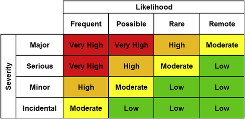
The result is called a “risk matrix.” Risk will be “low” in the bottom right corner of the risk matrix, where probability and consequence are low, and “very high” in the upper left corner of the matrix, where probability and consequence are high. Figure 2.23 shows a typical 4 × 4 risk matrix. A risk matrix does not need to be 4 × 4. They can be of different frequency–severity combinations; 5 × 5, 4 × 6, and 6 × 7 combinations as well as others are in use and can be effective risk management tools. The overall form of the risk matrix, the number of categories and what risk levels are deemed acceptable and unacceptable is determined by the management of the company or organization that uses the matrix. Because of the flexibility in the construction of the risk matrix, the method scales easily to the depth of analysis, the level of resolution desired and the range desired for consequences and event frequencies.

The risk matrix can be used qualitatively by having the risk assessment teams label events as “frequent” or “rare” with “major” or “incidental” consequences. It can also be used more quantitatively by precisely plotting specific frequency or consequence values on the matrix based on the underlying values and iso-risk curves used to construct the matrix.
A risk matrix can be applied to a problem of any scale as long as the matrix used for the analysis has been constructed appropriately. When using general levels like “frequent” or “rare” with “major” or “incidental” for a qualitative analysis, little to no scaling is required. When using the risk matrix in a more quantitative way, using actual frequencies and damages to place events on the matrix, the risk matrix can be applied to incidents of various scales by changing the definition of acceptable and unacceptable risk. When applying a risk matrix to a small, simple system, and acceptable risk level might be defined as $100/year or $200/year. For facility-wide scenarios, an acceptable risk level might be $1 million/year.
To use the risk matrix, a scenario or event is placed on the matrix according to its frequency of occurrence and severity of consequence. If the scenario falls into the “acceptable” zone, no action is required. If the scenario falls into the “conditionally acceptable” zone, action may or may not be taken depending of the nature of the hazard and the costs of risk reduction. If a scenario falls into the “unacceptable” zone, corrective action must be taken to reduce the risk of this event or scenario. Risk reduction measures can reduce the consequences of the event, the frequency of it, or both, as shown in Figure 2.24. Risk reduction measures are generally assumed to provide 1 or 2 orders of magnitude of risk reduction. Risk reduction measures and barriers should be added until the scenario or event falls in or near the acceptable zone.

2.4.7.3. HAZOP
The hazards and operability (HAZOP) study is a highly structured, inductive, procedure for identifying hazards in a facility. The HAZOP method is regarded as effective and is therefore widely accepted and implemented.
The HAZOP study generates process deviations by combining guide words with process parameters. Some guideword and parameter combinations are impossible or invalid and can therefore be ignored. Valid deviations are further analyzed and considered.
A complete HAZOP study for a process can take a very long time. to keep team members engaged and provide for effective brainstorming, it is best to break the study into sessions that last only a few hours. Meetings should only be held two or three times a week. As a result however, a full HAZOP study may require several weeks or months to complete. The HAZOP will follow a set of steps:
1. Collect process information including flow sheets.
2. Divide the process into nodes.
3. Select study team.
4. Determine the design intent of a node.
5. Select a process parameter.
6. Apply a guide word to the parameter to generate a deviation.
7. If the deviation is valid, determine possible causes and barriers.
8. Evaluate consequences and likelihood of the deviation.
9. Recommend actions be taken as appropriate if the expected consequences are too severe or if the current barriers are thought to be inadequate.
10. Record the results.
11. Repeat steps 6 through 10 for all guidewords with the selected parameter.
12. Repeat steps 5 through 11 with all relevant parameters in the node.
13. Repeat steps 4 through 12 for all nodes in the process.
This technique analyzes each element of a system for all the ways in which key operation parameters can deviate from the intended design operation conditions that could create hazards and safety problems. Typically, HAZOP studies are performed by analyzing the piping and instrument diagram (P&ID) of the facility. Usual parameters that are selected to perform this study are flow, temperature and pressure. Then a list of deviation keywords is used, for example, more of, less than, part of. Each of these parameters will create different situations that could lead to diverse outcomes and scenarios that could affect the integrity of the facility. Furthermore, this technique allows the identification of the safeguards and protection systems currently used and the ones that are needed to lower the risk to a tolerable level.
Documentation of the results is the most important part of the HAZOP study. Detailed documentation of the study will be needed later for review by auditors and to ensure that action items from the study are taken up and resolved. There are multiple methods for documenting the study results and the methods used vary from company to company and organization to organization. A common means of documentation is a form that lists the study node, parameter, guideword, causes, consequences, and recommended actions. An example of such a form is presented in Figure 2.25.
Similar to other methods discussed so far, there is no limit to the number of nodes used in a HAZOP or the size of the facility or system to which it can be applied. However, the difficulty of the analysis and the time required for it will scale roughly linearly with the number of nodes in the system. The more nodes, the longer the analysis will take, and a HAZOP on an entire plant can require a team to meet weekly or twice weekly for months to complete.
2.4.7.4. What-if analysis
This is a relatively informal method of analysis where-in the words “What-If” are placed in front of a number of possible events, failures or process upsets to form questions. The risk analysis team then determines the consequences and potential impacts on the process that the failure or upset might produce. Corrective and preventative actions are taken where necessary (Crowl and Louvar, 2011).
Some examples of questions include:
• What-if the flow of coolant to a heat exchanger is stopped?
• What-if the tubes in the heat exchanger leak?
• What-if a fire starts near the tank?
• What-if the concentration of the feed to the reactor is wrong?
• What-if the power fails?
• What-if water is accidentally introduced to the system?
Depending on the process, there are a potentially infinite number of questions that can be asked. However, the informal and unstructured nature of the what-if process requires that the analysis team know and ask the right questions. If a question is not asked, a hazard can be missed.
The informal nature of this method and its lack of structure make it likely ill-suited for analyzing large or complex systems, and this method is much more likely to be used either in the early stages of a design or for smaller systems.
The main purpose of this technique is to elaborate a list of what-if questions regarding the hazards and safety of the operations. As each question is answered, hazard scenarios are identified, and based on the team brainstorming, recommendations are developed specifying actions to be taken and additional studies to be performed to address risks.

2.4.7.5. Checklist
The checklist or process hazard checklist is a method generally used in the early stages of design and planning for the purposes of hazard identification and screening. Checklists can be useful for reminding operators or an analysis team of common or significant hazards in the process. The checklist design will vary depending on the purpose of the list and the scope of the analysis, which could be an entire process unit or a specific piece of equipment. Checklists suffer some limitations; however, as they can encourage a “check the box” mentality and will likely miss any hazards not on the list (Crowl and Louvar, 2011).
2.4.7.6. What-if/checklist
As the name suggests, this method combines elements of the what-if method and the checklist method to overcome some of the limitations of each. The checklist component seeks to ensure that some known significant hazards are thought of and addressed. The what-if component of the analysis encourages the analysis team to go beyond the checklist and look for additional hazards to the process.
2.4.7.7. Dow fire and explosion index
The Dow Fire and Explosion Index (F&EI) attempts to rate the hazards associated with the storage and handling of flammable and explosive substances in a purely systematic way that is as free as possible from independent judgment. The F&EI produces a score by which the relative size of the risk that a facility poses due to flammable hazards can be assessed. This is a relative measure that allows risks and processes to be compared. It is not an absolute or quantitative measure of risk.
The F&EI uses a material factor that is specific to the flammable material or mixture that is present in the unit or process. The material factor is then modified with multipliers, called penalty factors and credit factors, based on process characteristics, operating conditions, and safety precautions that have been put into place in the process. More detailed guidance on the F&EI can be obtained from Dow's Fire and Explosion Index Hazard Classification Guide, 7th edition, or from Crowl and Louvar (2011).
As might be inferred from the structure of the Dow F&EI analysis, it is designed to be applied to processes, not to individual pieces of equipment and not to large integrated facilities with multiple process trains. Examples of documenting the results of DFE&I are shown in Figures 2.26 and 2.27.
..................Content has been hidden....................
You can't read the all page of ebook, please click here login for view all page.