
Open source software for mass spectrometry and metabolomics
Abstract:
This chapter introduces open source tools for mass spectrometry (MS)-based metabolomics. The tools used include the R language for statistical computing, mzMine and KNIME. A typical MS-metabolomics data set is used for illustration and the tasks of visualisation, peak detection, peak identification, peak collation and basic multivariate data analysis are covered. A discussion of vendor formats and the role of open source software in metabolomics is also included. Example R scripts and KNIME R-nodes are shown, which should enable the reader to apply the principles to their own data.
4.1 Introduction
Mass spectrometry has advanced enormously since the invention of the first mass spectrometer built in 1919 by Francis Aston at Cambridge University [1, 2]. This first instrument is reported to have had a mass resolving power of 130. Less than a century later, many laboratories have at their disposal instruments capable of resolving powers in excess of 60 000 and a few specialist instruments may reach as high as 200 000. Technologies such as Time of Flight, Fourier Transform Ion Cyclotron resonance (FTICR) mass spectrometry and the new generation of ion traps (Orbitrap, Qtrap) have provided the researcher with unprecedented resolving power and potential.
In some ways it could be argued that the technology has moved faster than our ability to deal with the data. Despite such high-resolution instruments being available for several years, even instrument vendors’ software has struggled to keep pace with the potential abilities these instruments provide. In addition, the modern spectrometer places a huge strain on the computing hardware both in terms of storage and processing power. Our ability to process and make sense of such large data sets relies on cutting edge data visualisation and multivariate statistical methods.
Possibly for these reasons there have been a large number of open source projects started by researchers in mass spectrometry, chemometrics, metabolomics and proteomics. It is a rapidly developing area with many new innovations still to be made and one where collaboration is essential. We are moving into an age of research where no one person can possibly keep up with all the skills required. Instead communication and networking skills are becoming as important as scientific knowledge. Fortunately, the open source software community is an excellent forum for such collaborations.
In this chapter a few of these open source tools will be demonstrated.
4.2 A short mass spectrometry primer
As some readers of this book may be unfamiliar with mass spectrometry, here is a short explanation. (Mass spectrometry experts may wish to skip this section.)
A mass spectrometer can be described simply as a device that separates ions based on their mass to charge ratio. It is frequently used as a detector as part of a chromatography system such as high pressure liquid chromatography (HPLC), gas chromatography or used alone with samples being introduced from surfaces using laser desorption (MALDI) or directly from air (DART). Chemical samples are therefore introduced to the mass spectrometer as solutions, gases or vapours. The introduced substances are then ionised so that they may be deflected by electrostatic or magnetic fields within the spectrometer. Ions with different masses are deflected to different extents, so, by varying the deflection strength, a range of mass/charge ratios may be determined. The resulting plot of the molecular weight versus ion abundance is known as a mass spectrum.
From the pattern of masses detected, or from the exact mass, important clues to the structure of the original molecule may be determined. Molecules may travel through the instrument relatively intact or may fragment into smaller parts. A skilled mass spectrometrist is often able to infer the chemical structure of the original molecule by studying the fragments produced.
Some methods of mass spectrometry produce highly fragmented spectra, which represent ‘fingerprints’ characteristic of a particular molecule so searching against a stored library is possible. Modern multistage instruments are also able to deliberately fragment individually selected molecules by collision with low-pressure gas. This is known as MS/MS or sometimes MSn.
Rather surprisingly to an outsider, mass spectrometers often give poorly reproducible results between instruments, so spectra acquired from one instrument may not exactly match those from another. It is common practice to run large numbers of known molecules on a particular instrument to build a library specific to that instrument. The reason for the poor reproducibility is that ionisation of compounds is dependent on many factors and subtle changes between instruments can result in drastic differences in fragmentation and instrument response. Indeed ionisation of different molecules is unpredictable so that there is no direct relationship between the composition of a mixture and the response of the spectrometer. For quantitative work careful calibration of the mass spectrometer is required to determine the response of each chemical component.
With the newest high-resolution spectrometers, the precise mass of the compound can yield molecular formula information [3]. This is commonly termed ‘accurate mass measurement’. How can the mass of a compound lead to its molecular formula? To understand this, first a little theory is required.
4.2.1 Spectrometer resolution and accuracy
The resolution of a spectrometer is defined as the mass number of the observed mass divided by the difference between two masses that can be separated. For instance a resolution of 100 would allow a m/z of 100 to be distinguished from a m/z of 101.
The mass accuracy is defined in ppm (parts per million) units, and expresses the difference between an observed m/z and theoretical m/z. Today sub-ppm accuracy is not uncommon.
4.2.2 Definitions of molecular mass
In mass spectrometry, it is important to realise that the spectrometer will be measuring individual isotopes, so that, for instance, elements with two or more commonly occurring isotopes will be seen as multiple peaks (e.g. chlorine 35Cl, 37Cl).
The average mass of a molecule is the sum of the average atomic masses of the constituent elements. The average atomic mass is determined by the naturally occurring abundances of isotopes. For instance, carbon has an average mass of 12.0107(8) but is made up of 98.93% 12C (mass = 12 exactly) and 1.07% 13C (mass = 13.0033548378). The average mass is used in general chemistry but not mass spectrometry.
The monoisotopic mass is the sum of the most abundant isotopes in each molecule. For most typical organic molecules, this means the lightest of the naturally occurring isotopes. The monoisotopic mass will therefore represent the biggest peaks detected in the mass spectrometer. (However, for some heavier atoms this does not hold, for example iron (Fe) the lightest isotope is not the most abundant.)
The fact that the mass of an isotope is not exactly the sum of its neutrons and protons is due to an effect called the ‘mass defect’ and is due to the binding energy that holds the nuclei together. Some of the atomic mass is converted to energy according to the principle of relativity (E = mc2). Each isotope has a characteristic mass defect and this can be used to calculate an exact mass (for instance, see Table 4.1).
Table 4.1
| Isotope | Mass | Example |
| 12C | 12.00000 | C6H5NO2 |
| 1H | 1.007825 | |
| 14 N | 14.003074 | Monoisotopic = 123.032029 |
| 16O | 15.994915 |
Thus, by measuring the mass accurately on the spectrometer and matching that to a theoretical calculated mass, a molecular formula may be determined. Of course, many molecular structures are possible from a single formula and depending on the precision of the measurement there may be more than one molecular formula that fits the accurate mass. As molecular weight increases, the number of formulae that will fit a measured mass will increase for any given mass accuracy.
The nominal mass is the integer part of the molecular mass and was commonly used with older low-resolution spectrometers. Mass spectrometry is a complex subject. Reference [4] gives a good overview of the field.
4.3 Metabolomics and metabonomics
In this chapter the focus will be on the application of mass spectrometry to metabolomics and metabonomics. Both terms refer to the study of naturally occurring metabolites in living systems. ‘Metabolomics’ originally referred to the study of metabolites in cellular systems, whereas ‘metabonomics’ [5] referred to the metabolic response of entire living systems. Subsequently, confusion has arisen by the inconsistent adoption of either term [6]. These terms are often used interchangeably, so the term ‘metabolomics’ will be used in the text that follows.
In animal and human studies the study of metabolites is often by analysis of fluids such as urine, saliva, blood plasma or cerebral-spinal fluid. In this way the sampling may be non-invasive (urine/saliva) or at least non-lethal, and therefore allows the repeated collection of samples from the same individual. In plant metabolomics, a portion of the plant (or whole plant) is used. As removal of plant tissue is a disruptive event, it is rare that any repeated sampling will come from the same part of the plant tissue or even the same plant. Instead groups of plants are grown under carefully controlled conditions, with the assumption that the variation between individuals will be smaller than any treatment effects.
Extracts of the biological material are then presented to the analysis system where a ‘snapshot’ of the metabolites present in the sample is determined. This kind of global metabolite profiling is often called ‘untargeted analysis’ where the hope is that many compounds may be identified either by comparison with known, previously run compounds or that tentative identification by the mass spectrum or accurate mass may be made. This is in comparison to ‘targeted analysis’ where standard dilutions of known compounds are run in advance to determine the quantitative response of the instrument and to identify metabolites.
The consequence of untargeted analysis is that the quantitative information is relative between treatment groups. Within any particular sample the amounts of analytes detected may not represent their true concentration but a comparison of a control and treated sample for a particular peak will give a relative measure of that metabolite’s concentration between samples. Moreover, the data revealed by metabolomics represents a ‘snapshot’ at one point in time and gives no information about the dynamic flux of metabolites. For example, a metabolite showing a small concentration may in fact be transported in large quantities or one that shows high quantity may be produced very slowly but accumulates over time.
Identification of metabolites from the mass spectrum is one of the biggest challenges in metabolomics. Accurate mass and fragmentation patterns may assist in the determination of structure but for absolute certainty, preparative isolation of the substance followed by other methods such as NMR may need to be employed. Therefore in many studies it must be realised that identifications are somewhat tentative. This is not necessarily a major problem in hypothesis-generating research, but could potentially limit the use of untargeted methods in critical areas such as clinical diagnosis. Fortunately, robust multivariate methods may be used to fingerprint the combination of many metabolite signals in order to produce classifications with high levels of accuracy (low false positives and negatives) so the precise identification of individual components may be unnecessary for some applications.
4.4 Data types
Occasionally mass spectrometry data may be in the form of a mixed spectrum of all components in the case of ‘direct infusion’ where a sample is infused into an instrument. This is a simple 2D mass spectrum of mass/ charge ratio (m/z) and ion abundance (intensity).
More commonly data come from LC-MS, GC-MS or CE-MS where the complex mixtures are separated before being introduced to the mass spectrometer. The data which result are three-dimensional, having axes of mass/charge ratio (m/z), retention time and ion abundance (intensity).
4.4.1 Vendor formats versus open formats
The data from mass spectrometry, in common with many areas of analytical chemistry, are often saved in proprietary formats dictated by instrument vendors. There are several disadvantages with this situation, the difficulties of using a common software platform in labs with different manufacturers’ equipment, the hindrance of free interchange of data in the scientific community and the lack of ability to read archived data in the future. Although it is unlikely that instrument vendors will accept a common file format any time soon, many have the ability to export data into common open formats. There are also a number of converters available [7, 8], but care must be taken to preserve the integrity of the data.
MzXML [9], mzData and mzML [10, 11] are open, XML (extensible Markup Language)-based formats originally designed for proteomics mass spectrometric data. mzData was developed by the HUPO Proteomics Standards Initiative (PSI), whereas mzXML was developed at the Seattle Proteome Center. In an attempt to unify these two rival formats, a new format called mzML has been developed [11]. A further open format is JCAMP-DX [12], an ASCII-based representation originally developed for infra-red spectroscopy. It is seldom used for MS due to the size of the data sets. Finally, ANDI-MS is also open, and based on netCDF, a data interchange format used in a wide variety of scientific areas, particularly geospatial modelling. It is specified under the ASTM E1947 [13] standard. These are complemented by the wide variety of vendor-led formats in routine use in the field, the most common of which are .raw (Thermo Xcalibur, Waters/ Micromass MassLynx or Perkin Elmer); .D (Agilent); .BAF, .YEP and .FID(Bruker); .WIFF (ABI/Sciex) and .PKL (Waters/Micromass MassLynx).
The remainder of this chapter will demonstrate the use of open source tools to typical mass spectrometry situations.
4.4.2 Analysing mass spectroscopy data using R
A number of tools for mass spectrometry have been written in the R language for statistical computing [14]. Versions are available for Linux, Mac or Windows, making it compatible with a broad range of computing environments. One of the most convenient ways to run R is to use RStudio (http://rstudio.org/), which serves as integrated development environment. This software allows the editing of scripts, running commands, viewing graphical output and accessing help in an integrated system. Another very useful feature of R is the availability of ‘packages’, which are pre-written functions that cover almost every area of mathematics and statistics.
4.4.3 Obtaining a formula from a given mass
Our first example uses a Bioconductor package for the R language written by Sebastian Böcker at the University of Jena [15, 16]. The package uses various chemical intelligence rules to infer possible formula from a given mass. With this library, users are able to generate possible formulas from an input mass value and output this data via the command decomposeMass as shown below.
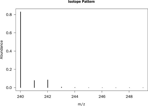
Subsequently, a formula can be selected and the isotopic distribution calculated using the getMolecule command. Plotting as a graph produces the output shown in Figure 4.1 representing the composition cystine with two sulphur atoms that have four isotopes 32S (95.02%), 33S (0.75%), 34S (4.21%) and 36S (0.02%).
4.4.4 Data visualisation
A vital part of data analysis is the visualisation of data, it is good practice to check the data visually for instrumental problems such as drift or baseline shifts. The XCMS package may be used for this purpose.
Examining a LC-MS spectrum in XCMS
The XCMS [16–20] package was written at the Scripps Center for Metabolomics and Mass Spectrometry and is now provided as part of the Bioconductor R package [15]. XCMS can be used to display the results of an LC-MS scan using a few straightforward steps. In the example, data from a single LCMS run are loaded into an ‘xcmsRaw’ object designated x1. The content and structure of this R object are viewed in order to extract data for plotting.
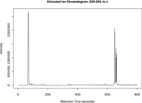
We can then use various commands to determine the start and stop times, mzrange and generate the TIC (total ion chromatogram) plot, shown in Figure 4.2. It is also possible to output the raw data as a retention time versus m/z versus intensity table as a CSV file.
The mass spectrum may also be plotted using the plotScan function:
where scan is the scan number, ident allows annotation of the peaks interactively with the mouse, see Figure 4.3 as an example.

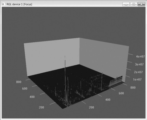
For a global overview of the LC-MS scan, a rotatable 3D image can be generated via the ‘plotSurf’ command within the RGL package [22], as shown in Figure 4.4. Although only a few elementary features of XCMS have been shown here, XCMS is a comprehensive metabolomics processing package [19–21] and there are many good tutorials [23].
Visualising an LC-MS run in R is useful but lacks a certain degree of interactivity. Another open source MS package is mzMine [24–26] developed at Okinawa Institute of Science and Technology, Japan and VTT Finland. It is a Java-based program and is therefore platform-independent. mzMine works with a rich set of file types including Net CDF, mzData, mzML, mzXML, Xcalibur Raw files and Agilent CSV files. (For the Thermo Xcalibur files it is necessary either to have the Thermo Xcalibur software installed on the same machine or to have downloaded and installed the free ThermoMSFilereader software [27].)
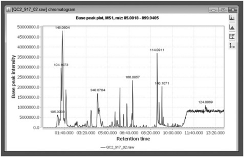
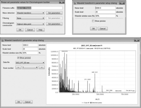
One of the great advantages of mzMine is its interactivity. Importing and processing the data is achieved using standard graphical file dialogs. For instance, the TIC visualiser produces a high-quality spectrum plot shown in Figure 4.5. The plot is fully zoomable and interactive, and double clicking a peak leads to its mass spectrum and associated data.
Peak detection is enabled using the chromatogram builder that has several different peak detection methods. Figure 4.5 demonstrates the use of the peak-list Wavelet method where the threshold for peak detection in the mass dimension and other options can be interactively adjusted. The ultimate aim is to create a set of parameters able to distinguish between true peaks and irrelevant/noisy features. Other options for peak detection in the mass dimension are Centroid (for previously centroided data), and Exact Mass Detector (which defines the peak centre at half maximum height), Local Maximum (simple local maxima) and Recursive Threshold (for noisy data).
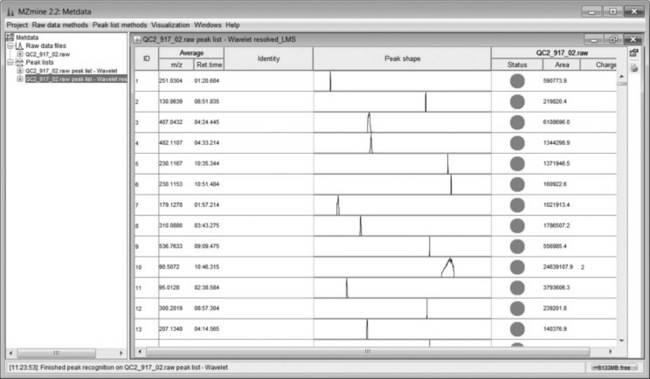
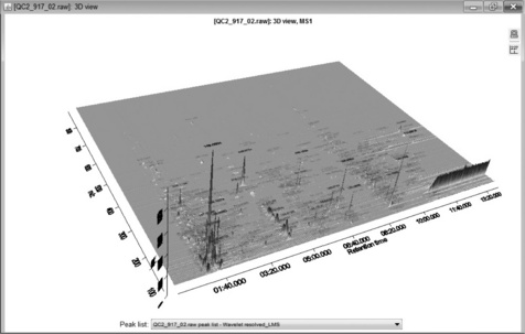
The peak list comprises a series of ion chromatograms taken at each mass channel detected in the chromatogram builder. Some ion chromatograms may contain more than one peak so a second peak deconvolution stage is required. Chromatogram deconvolution has several different methods to choose from, here local minimum search was used. This method searches for local minima in partially overlapping peaks and works well for chromatograms with well-defined peaks and low noise. Alternative methods are simple Baseline Cut-Off (threshold), Noise Amplitude (detects baseline noise amplitude) and Savitsky-Golay (standard peak detection method using second derivatives). After this step, mzMine produces a resolved peak list with one peak per row as shown in Figure 4.7. These data can be further explored by visualisation as a 3D plot (Figure 4.8) or 2D-Gel view. The 3D view is particularly useful as the detected peaks from a peak list are shown on the plot, which enables a visual check that peaks have been found correctly. Alternatively, several peak lists may be obtained by varying the detection parameters and visualised in the 3D view, the aim being to recognise the main peaks without excessive detection of baseline noise.
4.5 Metabolomics data processing
In metabolomics a number of samples are measured, resulting in a 3D LC-MS or GC-MS scan for each sample. Typically, this will consist of control, treated and repeated standard samples. The aim of metabolomics processing is to combine these scans together so that the relative amounts of metabolites occurring in all samples may be compared. The combination of data has to be done in a consistent way over all the data sets, and problems have to be accounted for such as small retention time drifts.
4.5.1 Processing a metabolomics data set in mzMine
Aside from the peak detection and data display features demonstrated above, mzMine is primarily a tool for metabolomics and has a number of useful features to support the extensive data processing required. The batch mode tool allows a chain of processes to be created; a very useful feature with large data sets as the processing can be set to run overnight in unattended operation. Furthermore, once the parameters for a particular operation have been configured, mzMine remembers the last used settings such that they may be applied across all samples in the study.
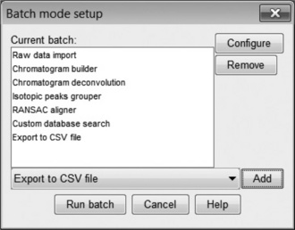
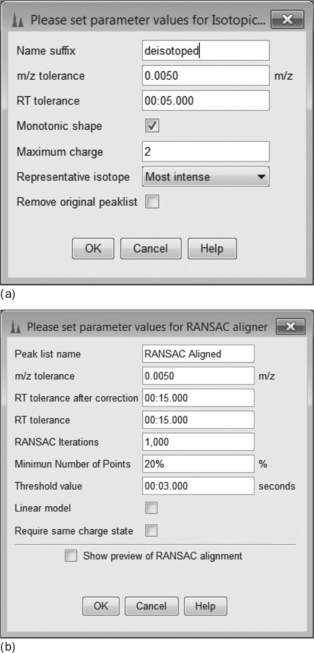
An example of a complete metabolomics workflow is shown in Figure 4.9. Each item in the list is associated with an operation from the mzMine menu, each with its own parameter settings dialog box. First (Figure 4.10(a)), the Isotopic Peaks Grouper is configured to find all 13C peaks and groups the area with the main 12C peak. Next (Figure 4.10(b)), the peaks are aligned using the RANSAC [28] Peak aligner, which is a method to join all the separate peak lists into one master list, accounting for both linear and non-linear deviations in retention time. An alternative is the simple Join aligner, which uses mz and RT windows. Because many small, possibly spurious, peaks may be detected in single runs, the combined table can be constrained to entries where there are a minimum of, say, 20 occurrences of that peak. Figure 4.10(c) shows how this is configured in mzMine. Finally (Figure 4.10(d)), in order to identify the peaks, a custom database of accurate mass/retention times measured on standard compounds is used. This library is simply a comma separated value file (.CSV) listing the mz, RT, molecular formula and name of each metabolite. The retention times are determined by the previous injection of standard samples onto the system. There are also options to search online databases such as ChemSpider, KEGG, METLIN, etc., but the hits are often rather promiscuous returning many research chemicals, drugs and mammalian metabolites. These may be irrelevant and misleading when the experiment concerns a limited, defined space, such as plant metabolites for example.
Once all the stages are configured satisfactorily it is possible to run the operations in batch mode. This can take some time and having a multicore processor is useful as mzMine is multithreaded. For the small example data set illustrated, this operation took approximately 5 minutes (PC = HP Zeon Z600 8-core 2.4 GHz workstation with 8 GB RAM running Windows 7, 64 bit). It is not uncommon in our laboratory to run analyses that take many hours of overnight operation for a typical metabolomic study. The final step in the workflow is an Export to CSV option that allows the export of the final spreadsheet for downstream analysis.
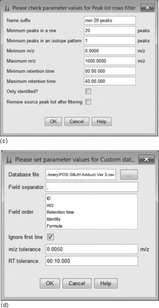
The end result of the data processing workflow is shown in Figure 4.11 ‘RANSAC Aligned min 20 peaks’. Peaks that are missing are shown as red spots in the table (shown boxed in the figure). As missing data is undesirable, mzMine can be configured to fill missing peaks using the regions defined in the peak table. This ensures a reading of real data which is preferable for later statistical analysis. mzMine has two main gap-filling options; ‘Peak finder’ and ‘m/z and RT range gap filler’. The former looks for undetected peaks in the same region as other scans, whereas the mz and RT gap filler simply finds the highest data point within the defined range.
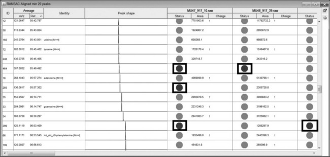
At this stage it is most likely that the data will be processed further in a commercial data analysis package, but there are a few basic data visualisation tools included in mzMine. Analysis options include: coefficient of variation (CV) analysis, log ratio analysis, principal component analysis, curvilinear distance analysis, Sammon’s projection and clustering. Use of these functions is illustrated below. (The data are taken from a metabolomic study on the ripening of fruits, comparing wild-type and non-ripening mutants, plus controls.)
Coefficient of variation analysis (Figure 4.12(a)) calculates the coefficient of variation of each peak and displays the result as a colour-coded plot. Log ratio analysis (Figure 4.12(b) ) looks at the difference between two groups. It is the ratio of the natural logarithm of the ratio of each group average to the natural logarithm of 2. Principal component analysis (Figure 4.12(c)) is a multivariate visualisation method. The first principal component shows a separation of the control samples from the wild type and mutant. The second principal component shows a vertical trend. This, at first glance, appears to be related to ripening, but on closer inspection the control samples also exhibit the same effect, showing that the variation is almost certainly due to spectrometer drift. The data have not yet been normalised to the internal standards which were spiked into the samples, an operation for the moment that has to be done outside mzMine. By removal of the control samples some separation of wild type from mutant was observed (not shown). Sammon’s projection (Figure 4.12(d)) is a nonlinear multidimensional scaling method which projects multidimensional data down to just two dimensions. It is a useful as a method to examine approximate clustering in data but offers no useful interpretability.
4.5.2 Other features in mzMine
There are many more features in mzMine, including some support for ms/ms data and extensive searching of external internet databases. More features are being added all the time, including several experimental baseline correction algorithms. Development in this area includes a raw data baseline correction module based on asymmetric least squares from the R package ptw: parametric time-warping [29] and an interface to the NIST MS Search [30] program to allow the use of mzMine for GC-MS data.
4.6 Metabolomics data processing using the open source workflow engine, KNIME
Data output from metabolomics software almost always requires further formatting before the data analysis stage. Procedures such as normalising the data to internal standards, or to total signal and subtotalling adducts are possible using spreadsheets and manual manipulation. The disadvantage of this approach is the ability to make unintentional errors and also the lack of transparency as to what was done to the data.
An alternative to this approach is to use a workflow tool which uses small data processing nodes linked together and therefore inherently documents the data set operations such as the open source project KNIME [31, 32]. Chapter 6 by Meinl, Jagla and Berthold describes applications of KNIME in chemical and bioinformatics. KNIME was developed by the Centre for Bioinformatics and Information Mining at the University of Konstanz and is based on the Eclipse platform for Java [33]. The KNIME software comes with a number of standard nodes but also there is a growing community of both commercial and open source developers writing new nodes for many data processing tasks. Included in KNIME are a number of statistical and data mining tools as well as data manipulation nodes. One of the really useful features is the support for writing code snippets in R, Java, Perl or Python, so if a KNIME node is not available for a particular application it is possible to write workarounds. Two examples of using KNIME and R for common metabolomics workflows are shown below.
4.6.1 Componentisation using mzMine
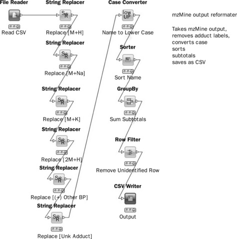
The first workflow will process the output of mzMine and componentise the identified metabolites. In other words, all identified adducts of a metabolite will be summed together in order to produce a component table. If, for instance, citric acid occurs as both [M + H], [M + Na] adducts then the workflow will add those peaks together. The actual workflow as seen in the KNIME GUI is shown in Figure 4.13. This workflow reads a CSV file, replaces adduct strings, converts all names to lowercase then subtotals the spreadsheet. In fact, in a spreadsheet such as Excel, string replacement and subtotalling are quite involved procedures and with large data sets the subtotalling may take a long time. In contrast, the KNIME workflow takes seconds to run and will run in a consistent manner eliminating manual processing errors. The workflow is constructed using various nodes. For example, the String Replacer node replaces any occurrence of a text (such as [M + H]) in the Name column. The Group By node groups rows by the Name column, here aggregations such as mean and sum of row subsets can be performed. The output is a CSV file with only the summed, identified metabolites in alphabetical order.
4.6.2 Internal standard normalisation using KNIME and R
In a typical metabolomics experiment, it is standard practice to include isotopic internal standards (such as d4-alanine, d5-phenylalanine) which Internal Standard and Total Signal Normalisation are spiked into the solvent used to dissolve freeze-dried plant material. The reason for this is to ensure there is a constant amount of standard in each sample so that instrumental response may be normalised. This avoids amplitude-based errors such as instrument drift, sample dilution or concentration. A KNIME workflow (Figure 4.14) can be created that identifies internal standards, averages the values and then divides each row in the original data by the internal standard. Although KNIME has many nodes for data manipulation, as yet there are none that allow mathematical functions to be applied to rows or columns within a data set so a custom R node (Labelled ‘R-Snippet’) can be used in order to do the division.
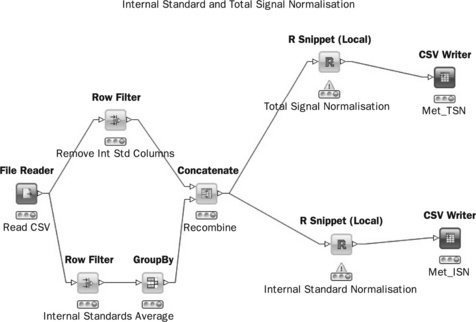
In cases where internal standards are not available several other methods are possible, one of the most common being total signal normalisation where each observation is divided by the total signal for that observation. In this way dilution effects may be eliminated. As with all normalisation methods, it is helpful to study replicate or pooled samples to see the effect of normalisation. If correctly normalised these samples should cluster into a tight group.
4.7 Open source software for multivariate analysis
Metabolomics data consist of very large numbers of variables and relatively few observations. Such data are inherently co-linear, which leads to the use of chemometric techniques that can handle highly correlated data by using latent variable methods [34]. These methods [35] include principal components analysis (PCA), principal components regression (PCR), Projection to latent structures (PLS), PLS discriminant analysis (PLS-DA), orthogonal PLS (OPLS®) [36, 43, 44], orthogonal PLS discriminant analysis (OPLS-DA®) [37] and kernel OPLS (K-OPLS) [38].
Once the data have been formatted and normalised, it is commonly analysed interactively in a commercial multivariate analysis package. However, the world of open source does offer some multivariate tools, mainly in the R language. There are several chemometrics packages for R.
![]() Chemometrics with R from the book Chemometrics with R – Multivariate Data Analysis in the Natural Sciences and Life Sciences by R Wehrens [39]. This package contains PCA and MCR routines.
Chemometrics with R from the book Chemometrics with R – Multivariate Data Analysis in the Natural Sciences and Life Sciences by R Wehrens [39]. This package contains PCA and MCR routines.
![]() Chemometrics. This package is the R companion to the book Introduction to Multivariate Statistical Analysis in Chemometrics by K Varmuza and P Filzmoser (2009) [40]. This includes PCA, PLS, clustering, self-organising maps and support vector machines.
Chemometrics. This package is the R companion to the book Introduction to Multivariate Statistical Analysis in Chemometrics by K Varmuza and P Filzmoser (2009) [40]. This includes PCA, PLS, clustering, self-organising maps and support vector machines.
![]() pls by R Wehrens and B-H Mevik [41]. Contains both PLS and PCR methods. This package is easily adapted for PLS-DA using a categorical Y variable denoting class membership (i.e. 0 = control 1 = treated).
pls by R Wehrens and B-H Mevik [41]. Contains both PLS and PCR methods. This package is easily adapted for PLS-DA using a categorical Y variable denoting class membership (i.e. 0 = control 1 = treated).
![]() pcaMethods [42], initiated at the Max-Planck Institute for Molecular Plant Physiology, Golm, Germany. Now developed at CAS-MPG Partner Institute for Computational Biology (PICB) Shanghai, P.R. China and RIKEN Plant Science Center, Yokohama, Japan. pcaMethods has a number of alternative PCA methods for missing data including NIPALS and support for cross-validation.
pcaMethods [42], initiated at the Max-Planck Institute for Molecular Plant Physiology, Golm, Germany. Now developed at CAS-MPG Partner Institute for Computational Biology (PICB) Shanghai, P.R. China and RIKEN Plant Science Center, Yokohama, Japan. pcaMethods has a number of alternative PCA methods for missing data including NIPALS and support for cross-validation.
![]() Kopls [38]. An implementation of the kernel-based orthogonal projections to latent structures (K-OPLS) method for MATLAB and R. The package includes cross-validation, kernel parameter optimisation, model diagnostics and plot tools.
Kopls [38]. An implementation of the kernel-based orthogonal projections to latent structures (K-OPLS) method for MATLAB and R. The package includes cross-validation, kernel parameter optimisation, model diagnostics and plot tools.
4.7.1 Important considerations with multivariate analysis
The most critical aspect of multivariate analysis is the ability to estimate the predictive power, or model stability. This is usually implemented using cross-validation [45] where some data are sequentially left out of the model and the model re-calculated. The left-out data are then estimated from the model and the differences are summarised in a parameter called Q2, the predictive variance. Without an estimate of predictivity, there is no objective way to estimate the optimum number of components or even if any components are actually predictive at all. The variance explained or R2 of a model will keep increasing with every component and so there is a great danger of overfitting the model if this is the only criterion used to judge the model.
The ability to estimate predictivity becomes of paramount importance when using supervised methods such as PLS-DA. Without the measure of Q2 it may be possible to get discriminant models which are effectively worthless, for example getting separations with random data [45]. In addition to cross-validation, permutation testing is also a highly effective
method of detecting overfit [46]. A second critical feature of multivariate methods is the use of the NIPALS [47] and related algorithms [35], which are able to handle small amounts of missing data without resorting to possibly misleading imputation (guessing) methods. Models are built with the data that are present, effectively ignoring the missing parts. Only some of the R packages implement cross-validation and missing value tolerance. Two of these are pcaMethods [42] and kopls [38].
4.8 Performing PCA on metabolomics data in R/KNIME
The pcaMethods package contains all required functionality in order to perform a simple PCA analysis. The input is an internal standard normalised data set as described in the previous section. A KNIME workflow to perform this analysis is shown schematically in Figure 4.15 and serves as a useful container for a number of small R scripts.
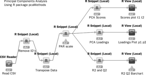
The PAR Scale node is a wrapper around R package pcaMethods, in this example, using Pareto scaling. (Pareto scaling is commonly applied to ‘omics data sets and is the division of mean centred variable columns by the square root of the standard deviation. It up-weights medium scale features without excessive increases in baseline noise.)
Alternatively, if scaling to unit variance is required the following code may be used.
Next, PCA scores are calculated using the NIPALS algorithm using pcaMethods.
The R View node provides the ability to produce R plots. The code below sets up a graph, colours the points according to class and plots the first two scores from the PCA node output.
To produce the loadings plots, the PCA model is recalculated to obtain the loadings and R View is used to plot the loadings.
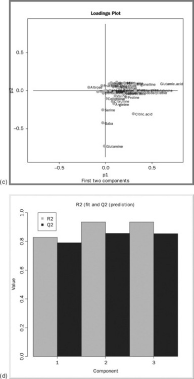
Finally, the R2 (Variance explained) and the Q2 (Predictive variance) are calculated via the following R code.
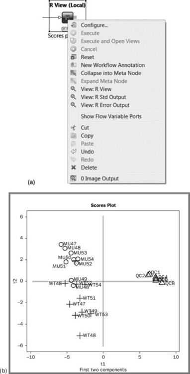
The output of the R View nodes may be seen by right clicking the node and selecting View: R View (Figure 4.16(a)). The PCA scores plot (Figure 4.16(B)) is shown in the output from the first RView node. The plot shows the improved clustering of the quality control samples after the internal standard normalisation (the cluster of triangles on the right hand side). Some, but not complete, separation in the two plant genotypes is seen. A new model containing just the plant samples would be the logical next step in the analysis. Figure 4.16(c) shows the loadings plot, which shows the pattern of the metabolites corresponding to the patterns observed in the scores plot. It appears that glutamine, gaba and citric acid are higher for the WT fruits, and glutamic acid is higher in the controls. Figure 4.16(d) shows the model is predictively sound as both the variance explained (R2) and predictive variance(Q2) are high.
Further possibilities for analysis may entail the use of the pls package for PLS-DA replacing the Y variable with class membership (0 or 1) for the genotypes or the more sophisticated kopls. This exercise is left for the reader to complete using the general principles outlined above.
4.9 Other open source packages
There are many more useful packages being developed for mass spectrometry and ‘omics data processing. For example, TOPPView is a viewer from the OpenMS proteomics pipeline for the analysis of HPLC/ MS data [48]. A full tutorial is available [49]. Cytoscape [50, 51] is an open source platform for network visualisation with good connectivity to bioinformatics resources. Network features such as node and edge parameters may be visualised in many ways, for instance levels of detected metabolites may be superimposed on a biological network. There is also an easy to follow tutorial available [52]. Ondex [53] is another data integration platform, which is designed to integrate diverse data sets and has a number of graph visualisation methods.
Finally, no discussion of metabolomics and mass spectrometry would be complete without mentioning the vast amount of data that studies are capable of producing. Although original data are often stored in instruments or dedicated LIMS systems, data modelling produces many types of intermediate data files. Many laboratories are resorting to backing up data onto high-capacity USB drives for storage or transfer. Although Linux users are in the fortunate position of having good operating system support for backups, Cobain Backup 8 [54] is an excellent open source program for automating backup of data in Windows. It is able to run either as a background service or an application and can schedule backup jobs to be started at daily or weekly intervals. The software supports FTP transfers and contains several methods of compression and strong encryption.
4.10 Perspective
As previously mentioned, the ‘omics technologies are developing at a rapid pace and the open source world is playing a valuable role in plugging the gap between newly developed academic methods and commercial vendors’ software. Many innovative and imaginative software packages are being developed, indeed since first writing this chapter the author has become aware of three more metabolomics packages namely MAVEN [55], R ‘Metabonomic’ Package [56] and Automics [57], the former for LC-MS and the latter two for NMR metabolomics.
Some issues with open source are difficult to use interfaces, experimental or buggy features, fragmentation of effort and poor availability of training materials. However, the growth of video-based training is beginning to improve the ease of use.
Another concern is the abandonment of projects. However, unlike commercial software, the source code is available so it is always possible to inspect, revive and adapt code which is no longer developed. Security is another concern, but as the code is under open scrutiny there should be less reason to fear open source than closed software.
One area that is frequently talked about, especially by commercial vendors, is the ‘lack of technical support’ with open source software. In our experience we have found completely the opposite. The open source community is very responsive to queries and more often than not bugs are fixed within days rather than the often months or years taken by commercial organisations. Active contribution to the projects also generates a lot of goodwill and need not be limited to programming skills as documentation and tutorials are highly valued.
Quite where the rise of open source in science leaves commercial software vendors is an interesting question. Having worked both in the software business and as an end user in industry, I can see advantages and disadvantages to both open and closed source products. The value of easy-to-use, well documented, validated and tested products that commercial vendors offer may often be underestimated. High licence fees may not look so high after considering the extra time needed to implement and learn less well-documented products (discussed in more detail by Thornber in Chapter 22). However, these costs are frequently hidden so that free open source packages may look very attractive from a budget holder’s point of view. Also, the ability to customise and tailor software exactly to your own needs is a big benefit that is seldom available with commercial products.
One area in which commercial vendors still have a key role is the of use of data analysis tools in regulated environments. Extensive software validation is a costly exercise and currently commercial software vendors take this responsibility and worry away from the customer, naturally in exchange for licence fees. For those interested in this area, Chapter 21 by Stokes discusses this in much more detail.
In more research-based areas, open source solutions may have an edge over commercial software due to the openness of algorithms. There have been recent moves to make data analysis more transparent by embedding algorithms inside publications using tools such as R and Sweave [58]. There has been much discussion about ‘reproducible research’ [59, 60], where not only the data but also the methods used for analysis are freely available. This could be a valuable contribution to the aim of being able to reproduce complex ‘omics analyses.
Open source is certainly a challenge to the commercial software world and we have seen the rise of many new business models, such as open community development with support, consultancy and training being run as commercial services. One area of relevance to Metabolomics is the provision of online services [61]. How open and free these type of services are likely to remain if massive transfers of data occur, remains to be seen. Commercial cloud computing solutions may emerge; but data security is of great concern to commercial organisations. I believe most commercial researchers would be very uneasy about transferring sensitive metabolomics data, particularly in highly commercial areas such as disease diagnosis or regulatory studies.
Lastly in the data analysis area, it appears so far only commercial vendors have been able to produce truly interactive data analysis tools. Products such as SIMCA-P, Unscrambler and JMP allow interactive plotting, data exclusion, filtering, transformation and many other manipulations. These operations are essential to any large-scale data analysis task where several rounds of quality control and data cleanup must be performed. To date, most of the data analysis tools in the open source are script-based and offer little opportunity for truly interactive analysis. Two packages which are attempting to make R more user-friendly and interactive are Rattle [62, 63] and GGobi [64, 65] but to date these have focussed more on ‘machine learning’ for business applications rather than chemometrics. (In general terms, machine learning algorithms require many more observations and fewer variables than are encountered in metabolomics, hence the preferred use of Chemometric methods, which are specifically designed for ‘wide’ data sets.) It will be interesting to see if any open source interactive tools will be developed in the future.
4.11 Acknowledgments
The author would like to thank the following people for help past and present who have guided the way through difficult and challenging territory. No single person can possibly know everything in today’s cross-disciplinary world of science but knowing who to ask is a great help!
Dave Portwood, Mark Seymour, Mansoor Saeed, Mark Forster, Charlie Baxter, Stuart Dunbar at Syngenta, Tomas Pluskal, Chris Pudney and all the mzMine developers, Tim Ebbels, Richard Barton, Elaine Holmes, Hector Keun at Imperial College, Svante Wold, Lennart Eriksson, Erik Johansson, Johan Trygg, Thomas Jonsson, Mattias Rantalainen, Oliver Whelehan and all my friends from Umea and Umetrics, Charlie Hodgman, Graham Seymour at Nottingham University, Madalina Oppermann at Thermo Instruments, Michael Berthold at Knime, Stephan Neumann at IPB-Halle and Stephan Biesken at the EBI.
4.12 References
[1] Griffiths, J. A Brief History of Mass Spectrometry. Analytical Chemistry. 80(15), 2008.
[2] http://en.wikipedia.org/wiki/History_of_mass_spectrometry.
[3] Webb K, Bristow T, Sargent M, Stein B and ESPRC National Mass Spectrometry Centre. Methodology for Accurate Mass Measurement of Small Molecules Best Practice Guide. Swansea UK. ISBN 0-948926-22-8.
[4] de Hoffmann, E., Stroobant, V. Mass Spectrometry: Principles and Applications, 3rd Edition. Wiley; September 2007. [ISBN: 978-0-470-03310-4].
[5] Nicholson J K. Molecular Systems Biology 2:52 Global systems biology, personalized medicine and molecular epidemiology. Department of Biomolecular Medicine, Faculty of Medicine, Imperial College London, South Kensington, London, UK doi:10.1038/msb4100095
[6] Robertson, D.G., Metabonomics in Toxicology: A Review 1. Toxicological Sciences 2005; 85:809–822, doi: 10.1093/toxsci/kfi102.
[7] http://tools.proteomecenter.org/wiki/index.php?title=Formats:mzXML.
[8] http://en.wikipedia.org/wiki/Mass-spectrometry_data_format.
[9] Pedrioli, P.G., Eng, J.K., Hubley, R., et al. A common open representation of mass spectrometry data and its application to proteomics research. Nat Biotechnol. 2004; 22(11):1459–1466.
[10] Deutsch, E.W. mzML: A single, unifying data format for mass spectrometer output. Proteomics. 2008; 8(14):2776–2777.
[11] http://www.psidev.info/index.php?q=node/257.
[12] Hau J, Lampen P, Lancashire RJ, et al. JCAMP-DX V. 6.00 for chromatography and mass spectrometry hyphenated methods (IUPAC Technical Note 2005).
[13] ASTM E1947–98(2009) Standard Specification for Analytical Data Interchange Protocol for Chromatographic Data DOI: 10.1520/E1947-98R09.
[14] R Development Core Team. R: A Language and Environment for Statistical Computing. R Foundation for Statistical Computing Vienna, Austria 2011 ISBN 3-900051-07-0 http://www.R-project.org.
[15] Gentleman, R., Carey, V.J., Bates, D.M., et al. Bioconductor: Open software development for computational biology and bioinformatics. Genome Biology. 2004; 5:R80.
[16] Neumann, S., Pervukhin, A., Bocker, S. Mass decomposition with the Rdisop package. Leibniz Institute of Plant Biochemistry. Department of Stress and Developmental Biology, Bioinformatics, Friedrich-Schiller-University Jena; 2010. [April 22,].
[17] Bocker, S., Letzel, M., Liptak, Z., Pervukhin, A. SIRIUS: Decomposing isotope patterns for metabolite identification. Bioinformatics. 2009; 25(2):218–224.
[18] Tautenhahn, R., Bottcher, C. Neumann S. BMC Bioinformatics: Highly sensitive feature detection for high resolution LC/MS; 2008.
[19] Smith, C.A., Want, E.J., Tong, G.C. Abagyan R and Siuzdak G. Processing Mass Spectrometry Data for Metabolite Profiling Using Nonlinear Peak Alignment, Matching, and Identification. Analytical Chemistry: XCMS; 2006.
[20] Smith, C.A., Want, E.J., Tong, G.C., et al, Metltn XCMS: Global metabolite profiling incorporating LC/MS filtering, peak detection, and novel nonlinear retention time alignment with open-source software. 53rd ASMS Conference on Mass Spectrometry. San Antonio, Texas, June 2005.
[21] Benton, H.P., Wong, D.M., Trager, S.A., Siuzdak, G., XCMS2: Processing Tandem Mass Spectrometry Data for Metabolite Identification and Structural Characterization. Analytical Chemistry. 2008.
[22] www.neoscientists.org.
[23] http://metlin.scripps.edu/xcms/faq.php.
[24] Pluskal, T., Castillo, S., Villar-Briones, A., Oresic, M. MZmine 2: Modular framework for processing, visualizing, and analyzing mass spectrometry-based molecular profile data. BMC Bioinformatics. 2010; 11:395.
[25] Katajamaa, M., Miettinen, J., Oresic, M. MZmine: Toolbox for processing and visualization of mass spectrometry based molecular profile data. Bioinformatics. 2006; 22:634–636.
[26] Katajamaa, M., Orešič, M. Processing methods for differential analysis of LC/MS profile data. BMC Bioinformatics. 2005; 6:179.
[27] http://sjsupport.thermofinnigan.com/public/detail.asp?id=586.
[28] Fischler, M.A., Bolles, R.C., 981. Random sample consensus: a paradigm for model fitting with applications to image analysis and automated cartography. Commun ACM. 1981;24(6):381–395, doi: 10.1145/358669.358692. http://doi.acm.org/10.1145/358669.358692
[29] Boelens, H.F.M., Eilers, P.H.C., Hankemeier, T. Sign constraints improve the detection of differences between complex spectral data sets: LC-IR as an example. Analytical Chemistry. 2005; 77:7998–8007.
[30] http://chemdata.nist.gov/mass-spc/ms-search/.
[31] http://www.inf.uni-konstanz.de/bioml2/publications/Papers2007/BCDG+07_knime_gfkl.pdf.
[32] http://www.knime.org/.
[33] http://www.eclipse.org/.
[34] Eriksson, L., Antti, H., Gottfries, J., et al. Using chemometrics for navigating in the large data sets of genomics, proteomics, and metabonomics (gpm). Analytical and Bioanalytical Chemistry. 380(3), 2004.
[35] Fonville, J.M., Richards, S.E., Barton, R.H., et al. The evolution of partial least squares models and related chemometric approaches in metabonomics and metabolic phenotyping. J Chemometrics. 2010; 24:636–649.
[36] Trygg, J., Wold, S. Orthogonal Projections to Latent structures (O-PLS). J Chemometrics. 2002; 16:119–128.
[37] Bylesjo, M., Rantalainen, M., Cloarec, O., et al. OPLS discriminant analysis: combining the strengths of PLS-DA and SIMCA classification. J Chemometrics. 2006; 20:341–351.
[38] Bylesjo, M., Rantalainen, M., Nicholson, J.K., et al. K-OPLS package: Kernel-based orthogonal projections to latent structures for prediction and interpretation in feature space (2008). BMC Bioinformatics. 2008; 9:106.
[39] Wehrens, R., Chemometrics with R: Multivariate Data Analysis in the Natural Sciences and Life Sciences (Use R).Springer, 2011. 9783642178405.
[40] Varmuza, K., Filzmoser, P. Introduction to Multivariate Statistical Analysis in Chemometrics. Boca Raton, FL: Taylor & Francis – CRC Press; 2009. [ISBN: 978–1420059472].
[41] Mevik, B.-H., Wehrens, R. The pls Package: Principal Component and Partial Least Squares Regression in R. Journal of Statistical Software. 2007; 18(2):1–24.
[42] Stacklies, W., Redestig, H., Scholz, M., Walther, D., Selbig, J. pcaMethods – a bioconductor package providing PCA methods for incomplete data. Bioinformatics. 2007; 23(9):1164–1167. [Epub 2007 Mar 7.].
[43] Trygg J, Wold S. Umetrics AB No. 10204646 filed on 22 February 2001.
[44] OPLS Trademark 78448988 Registration Number: 3301655 Filing Date: 12 July 2004.
[45] Westerhuis, J.A., Huub, C.J., Hoefsloot, S., et al. Assessment of PLSDA cross validation. Metabolomics. 2008; 4:81–89.
[46] Eriksson L, Trygg J, Wold S. SSC10 CV-ANOVA for significance testing of PLS and OPLS® models. Special Issue: Proceedings of the 10th Scandinavian Symposium on Chemometrics. Journal of Chemometrics 22(11–12):594–600.
[47] Wold, H., Lyttkens, E. Nonlinear Iterative Partial Least Squares (NIPALS) Estimation Procedures. Bull ISI PLS; 1969.
[48] Sturm, M., Kohlbacher, O. TOPPView: An Open-Source Viewer for Mass Spectrometry Data. J Proteome Res. 2009; 8(7):3760–3763.
[49] http://www-bs2.informatik.uni-tuebingen.de/services/OpenMS/OpenMS-release/TOPP_tutorial.pdf.
[50] Smoot, M.E., Ono, K., Ruscheinski, J., Wang, P.L., Ideker, T. Cytoscape 2.8: new features for data integration and network visualization. Bioinformatics. 2011; 27(3):431–432. [Epub 2010 Dec 12.].
[51] http://www.cytoscape.org/.
[52] http://cytoscape.wodaklab.org/wiki/CytoscapeRetreat2008/UserTutorial.
[53] http://www.ondex.org/.
[54] http://www.educ.umu.se/~cobian/cobianbackup.htm.
[55] Melamud, E., Vastag, L., Rabinowitz, J.D. Metabolomic Analysis and Visualization Engine for LC?MS Data. Analytical Chemistry. 2010; 82(23):9818–9826.
[56] Izquierdo-Garcia, J.L., Rodriguez, I., Kyriazis, A., et al, A novel R-package graphic user interface for the analysis of metabonomic profiles. BMC Bioinformatics 2009; 10:363, doi: 10.1186/1471-2105-10-363.
[57] Wang, T., Shao, K., Chu, Q., et al, Automics: an integrated platform for NMR-based metabonomics spectral processing and data analysis. BMC Bioinformatics 2009; 10:83, doi: 10.1186/1471-2105-10-83.
[58] http://www.stat.uni-muenchen.de/~leisch/Sweave/
[59] http://reproducibleresearch.net/index.php/RR_links.
[60] http://journal.r-project.org/archive/2010–1/RJournal_2010–1_Thioulouse~et~al.pdf
[61] https://xcmsonline.scripps.edu/.
[62] http://rattle.togaware.com/.
[63] Williams, G.J. Rattle: A Data Mining GUI for R. The R Journal. 2009; 2073–4859. [1/2. ISSN].
[64] http://www.ggobi.org/.
[65] Temple Lang, D., Swayne, D.F., DGGobi meets R: an extensible environment for interactive dynamic data Visualization. Proceedings of the 2nd International Workshop on Distributed Statistical Computing. 15–17 March, 2001 Vienna, Austria http://www.ci.tuwien.ac.at/Conferences/DSC-2001