
Integrated data analysis with KNIME
Abstract:
In this chapter the open source data analysis platform KNIME is presented. KNIME allows the user to create workflows for processing and analyzing almost any kind of data. There is a short introduction to KNIME and its key concepts such as nodes and views, followed by a short review of KNIME's history, and the origin and key aspects of its success today. Finally, several real-world applications of KNIME are presented. These examples include workflows from the fields of chemoinformatics and bioinformatics, and image processing. All these workflows apply freely available extensions to the basic KNIME distribution contributed by community members.
6.1 The KNIME platform
The Konstanz Information Miner (KNIME) has been developed by the Nycomed Chair for Bioinformatics and Information Mining at the University of Konstanz since 2004. KNIME is open source and since 2010 it has been licensed under GPLv3. Therefore, for researchers, at universities or in industry, it is a free yet powerful tool to perform all kinds of data analysis. Based on the Eclipse platform (and thus Java) it runs on every major operating system (Windows, Linux, and MacOS X, both 32bit and 64bit) and is very easy to install – all users need to do is download [1] and unpack an archive (which already includes Java).
With KNIME, the user can model workflows, consisting of nodes that process data, which is transported via connections between the nodes. A flow usually starts with a node that reads in data from some data source, usually text files, but databases can also be queried by special nodes. Imported data are stored in an internal table-based format, where columns have a certain data type (integer, string, image, molecule, etc.) and an arbitrary number of rows conforming to the column specifications. These data tables are sent along the connections to other nodes. In a typical workflow, the data will first be pre-processed (handling of missing values, filtering columns or rows, partitioning into training and test data, etc.) and then predictive models are built with machine learning algorithms such as decision trees, naive Bayes classifiers or support vector machines. A number of view nodes are available to inspect the results of analysis workflows, which display the data or the trained models in various ways. Figure 6.1 shows a small workflow with some nodes.
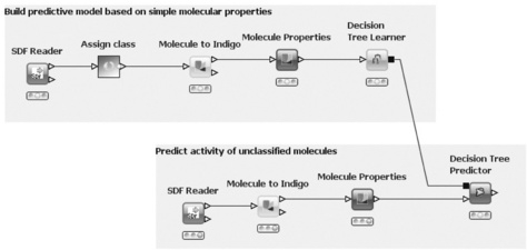
The figure also illustrates how workflows can be documented by use of annotations: in the upper part of the flow classified molecules are read in, properties are calculated, and finally a decision tree is built to distinguish between active and inactive molecules. The lower part reads unclassified molecules and predicts activity by using the decision tree model.
In contrast to many other workflow or pipelining tools, KNIME nodes first process the entire input table before the results are forwarded to successor nodes. The advantages are that each node stores its results permanently and thus workflow execution can easily be stopped at any node and resumed later on. Intermediate results can be inspected at any time and new nodes can be inserted and may use already created data without preceding nodes having to be re-executed. The data tables are stored together with the workflow structure and the nodes' settings. The small disadvantage of this concept is that preliminary results are not available as soon as possible as in real pipelining (i.e. when single rows are sent along and processed as soon as they are created).
Alternatively, many tasks performed via workflows can also be (often very simply) accomplished by applying simple spreadsheet programs or hand-written scripts. However, a workflow is a much more powerful method. In contrast to spreadsheets, it allows access to intermediate results at any time and can handle many more data types than just numbers or strings – to name only two advantages. In comparison to a set of scripts, a workflow is much more self-documenting, thus even non-programmers can easily understand which tasks are performed. Moreover, KNIME offers many more useful features, some of which we briefly describe in the following sections.
6.1.1 Hiliting
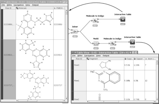
One of KNIME's key features is hiliting. In its simple form, it allows the user to select and highlight several rows in a data table with the result that the same rows are also hilited in all other views that show the same data table (or at least the hilited rows). This type of hiliting is simply accomplished by using the 1:1 correspondence between the tables' unique row IDs. There are, however, several nodes that completely change the input table structure and yet there is still some relation between input and output rows. A nice example is the MoSS node, which searches for frequent fragments in a set of molecules. The node's input are the molecules, the output the discovered frequent fragments. Each of the fragments occurs in several molecules. By hiliting some fragments in the output table, all molecules in which these fragments are contained are hilited in the input table. Figure 6.2 shows this situation in a small workflow. In this flow, public nodes from Indigo (see also below) are used to display the molecular structures.
6.1.2 Meta-nodes
Workflows for complex tasks tend to increase considerably in size. Meta-nodes are a practical way of structuring them. They encapsulate sub-workflows, which require several nodes to accomplish a certain task in the parent workflow. Meta-nodes can either be created as empty sub-workflows, to which other nodes are added, or a number of nodes in an existing workflow can be selected and collapsed into a meta-node. Meta-nodes can even be nested to arbitrary depths. Moreover, certain common tasks, such as cross-validation or feature elimination, which require more than one node are available as pre-configured meta-nodes in the node repository.
6.1.3 Loops
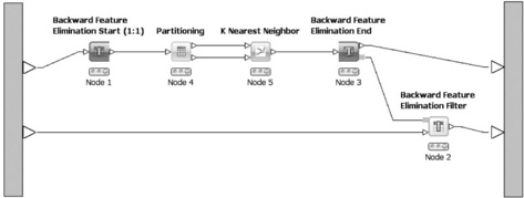
The workflows' conceptual structure is a directed acyclic graph, that is there are no loops from the output of one node to the input of one of its predecessors. Data flows strictly in one direction. However, there are cases in which the repeated execution of parts of the workflow with changed parameters is desirable. This can range from simple iterations over several input files, to cross-validation where a model is repeatedly trained and evaluated with different distinct parts of data and can include even more complex tasks such as feature elimination. In order to be able to model such scenarios in KNIME, two special node types are available: loop start- and loop end-nodes. In contrast to normal nodes (inside the loop), they are not reset while the loop executes, both nodes have access to its counterpart, and they can directly exchange information. For example, the loop end-node can tell the start-node which column it should remove at the next iteration or the start-node can tell the end-node whether or not the current iteration is last. Figure 6.3 shows a feature elimination loop in which the start- and end-nodes are visually distinguishable from normal nodes. The feature elimination model can subsequently be used by the feature elimination filter to remove attributes from the data table.
The node repository contains several predefined loops encapsulated in meta-nodes, such as a simple 'for' loop, which is executed a certain number of times, cross validation, iterative feature elimination, or looping over a list of files.
6.1.4 Extensibility
KNIME is an Eclipse-based application, which has two major implications. First, it is written in Java meaning that it runs on all major operating systems (Windows, Linux, MacOS X). Second, the Eclipse platform was designed to be highly extensible – as is KNIME. Developers can easily write their own extensions to KNIME by using the public API. Once packaged appropriately – either as ZIP files or as online update sites – users can quickly install (and uninstall) them into their existing KNIME installation by using the graphical update manager.
6.2 The KNIME success story
As already mentioned, KNIME initially started as a university project with a group of four people. One advantage about this kind of project is that it is relatively easy to find developers in the form of PhD students or student assistants who invest considerable amounts of time on the project. In the case of KNIME, one of the four people had already gained several years' experience as a professional software developer. However, it still took more than two years before the first version was ready for the public (28 July 2006). One big disadvantage of many university projects is the sustainability of the project: when developers leave – because they have graduated – they can only spend little if any time on further development, which often leads to the death of the project. There are two ways out of this dilemma. One way round this problem is to attract a large number of developers outside the group right from the beginning to ensure that when one developer leaves, another developer is there to step in and continue with the work. This, however, usually only works for very wide-spread projects such as the Linux kernel, the Apache web server, or the Secure Shell, for example. Another solution to the problem is to found a commercial company to take care of and continue with further development. A combination of both is possible of course.
For KNIME, the second option, the foundation of KNIME.com [2] in 2008, proved to be strategic to its success. Once the key people from the university group had completed their PhD, they switched to the company. Besides being in charge of further development of the open source KNIME core, the KNIME.com team is currently developing commercial extensions such as a KNIME server and cluster execution components. Another important focus of the company is to provide training courses for users and developers as well as support in case of problems. The university group continues to develop new nodes based on current research topics. Both parties collaborate well and ensure that the basic KNIME functionality is extended and new analysis methods are added.
Even though about 15 people are currently working on KNIME in both groups, it is obvious that they cannot develop solutions for all kinds of applications areas nor do they have the means to develop all the existing methods further in a given scientific area. Fortunately, two other parties jumped in. From the beginning there were commercial vendors (such as Schrodinger or Tripos) who integrated their existing tools into KNIME. The number of such companies has grown tremendously in recent years. A growing number of community members have also started developing extensions, which they provide free of charge to the community. Initially they were scattered over different locations, but since 2011 many of them are centrally hosted on the official KNIME server. This has benefits for the users, who have a central access point to obtain extensions for KNIME and do not need to search and collect them from various sources, while developers also benefit from the fact that they are provided with a source code repository as well as a nightly build service, a web page, and a discussion forum. At the time of writing, seven different projects exist in the KNIME Community Contributions [3] and many others are already in the queue. Remarkably, not all projects are from universities or other governmentally funded groups, but also come from industry.
6.3 Benefits of 'professional open source'
The term 'professional open source' stands for a business model where a vendor provides support and commercial extensions to an otherwise open source program. This concept was successfully pioneered by companies such as Red Hat or MySQL. In the same fashion, KNIME. com offers the 'KNIME Professional' package, which adds personal support and access to emergency patches in addition to the free open source version (see http://www.knime.org/products for details). This is especially useful when KNIME is used in production environments. To facilitate collaboration inside or between groups in a company, KNIME. com also provides the KNIME Team Space and the KNIME Server which enable (besides other features) easy sharing of workflows and meta-node templates.
Not only is the 'professional' aspect beneficial to (industry) users, but also the open source 'core' has several advantages for all user groups. First of all, the usage is completely free of charge, no matter how many computers it is installed on. This may not be an issue for some companies with regard to using the graphical user interface on a limited number of desktop computers, but as soon as it comes to deploying KNIME on a large compute cluster or even in a cloud, the benefits of open source and its licenses are obvious. The latter is especially interesting because KNIME can also be run in batch mode without a graphical user interface to execute pre-built workflows. This allows huge amounts of data to be processed on a large scale with no additional software costs.
Another aspect of KNIME's free accessibility is that many more people can easily use it and start to write extensions for their own or other freely available programs. These not only include Indigo [4], RDKit [5], or Imglib [6] as described in the next section, but also connectors to other well-known open source software programs such as the R statistics software and the Weka Data Mining suite, or integration of programming languages such as Perl or Python. Having access to such well-established software packages from inside KNIME is a benefit to all users, both in academia and industry.
6.4 Application examples
KNIME is used in many areas, such as finance, publishing, and life sciences. A private bank in Switzerland, for example, is applying KNIME workflows for customer segmentation based on investment philosophy and purchase behavior. A German publishing company is using KNIME to conduct propensity-to-purchase scoring and to look for early non-renewal indicators. A world-wide B2B-organization applies KNIME to perform needs and value segmentation of their customers to better plan campaigns via their sales force.
These are only a few examples of KNIME's usage in non-life science industries. However, the life sciences such as chemoinformatics and bioinformatics are the fields in which KNIME is currently used the most. Therefore the following example workflows deal with problems relevant to these areas. In order to use these workflows, one first needs to download and unpack KNIME [1]. As all workflows make use of nodes contributed by community members, you need to install the respective extensions from the Community Contributions [3].
All workflows are available on the public workflow server, which can be conveniently accessed directly from any KNIME installation.
6.4.1 Comparing two SD files with Indigo
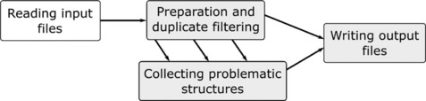
The following scenario depicts a common use case in chemoinformatics. A supplier delivers an SD file with new structures and the user wants to check whether these structures are already in the corporate database or if there are new structures that should be purchased. This task can be accomplished with the following KNIME workflow. As the workflow is too big to be shown on a single page in readable form, we have divided it into four different parts. The overall process is depicted in Figure 6.4.
The first part is shown in Figure 6.5 and is quite simple: first, it reads two SD files (e.g. the first containing the new structures from the vendor and the second containing the corporate database) with the SDF Reader, then adds a column indicating the source of each molecule with a Java Snippet node, and finally concatenates both tables.

This small workflow already shows two interesting concepts in KNIME. First, the SDF Reader has two output ports: the upper port provides a table with all the structures that have been successfully parsed and the second port contains a (possibly empty) table with structures that could not be parsed due to syntactic errors in the SD file. The reader node does not try to interpret the contents of the file but merely extracts the text representing each molecule into a cell of the output table. The interpretation is done by special conversion nodes (e.g. CDK, Indigo, Schrodinger, Tripos, etc.), which are more or less strict about the actual representation of a molecule. Second, the Concatenate node has so-called optional input ports. Usually, a node can only be executed if all input ports are connected, but for optional input ports this is not necessary. This makes perfect sense when concatenating tables because it frees the user from having to build a cascade of two-port concatenation nodes when there are several tables to combine.
The next part of the workflow deals with the preparation of the molecules. The Indigo [4] nodes are used for the whole filtering process. These nodes were recently contributed as open source by GGA Software and build on their Indigo chemical library.
In the first step (Figure 6.6), the SD records read in by the previous step are converted into the internal Indigo format. Molecules that cannot be converted, for example because of wrong stereochemistry or invalid atom types, are transferred to the second output port and added to the list of problematic structures (not shown). All remaining molecules are checked for correct valences and structures further down the pipeline. Structures failing the test are again added to the problematic structures. In the next step very small compounds (having a molecular weight of less than 10) are filtered out as uninteresting. Also, all structures that consist of several fragments are removed. This is necessary because in the next step (see Figure 6.7) canonical SMILES are generated, which cannot handle disconnected structures.
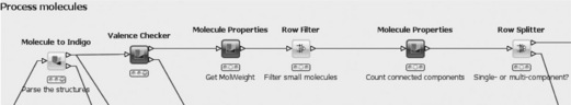
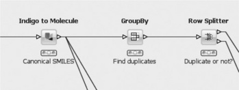
The most important step involves the Group By node, which groups all incoming rows based on the canonical Smiles string. In addition, it adds two columns to each canonical SMILES: a list of IDs that share the same SMILES, and the number of rows with that SMILES. The following row splitter is then used to divide the molecules into unique molecules (first output port) and duplicates (second output port) simply based on the number previously mentioned.
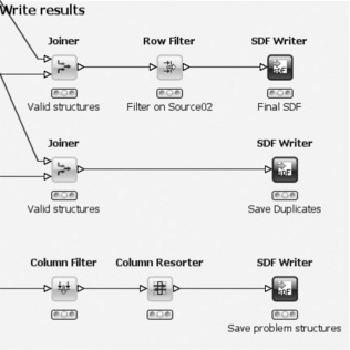
The last part of the workflow consists of writing the different sets of molecules to files (Figure 6.8). The upper row takes the unique molecules determined in the previous step and joins them with the table containing the converted molecules. This is necessary because they get lost during the group by operation (although this step can be omitted if one is only interested in the IDs of the SMILES). The converted molecules also provide a good 2D depiction for further inspection. The Row Filter node is important. It removes the unique molecules that come from the second input file. Assuming that this contains the pre-existing structures, all that is left after this node are the new structures. They are finally written into an SD file. The middle row of the workflow likewise saves all duplicate structures, whereas the bottom row saves all problematic structures that were gathered during the various preparation steps into another file (removing and resorting some properties for convenience before they are actually written to the file).
6.4.2 Enumerating amides with RDKit
The next workflow deals with reaction simulation, in particular the formation of amides by a two component reaction of amines and acids. Similar workflows are in use at Novartis and other pharmaceutical companies. This workflow makes use of the RDKit [5] nodes. A lot of functionality is provided from this well-known open source toolkit in KNIME. The concepts of quickforms and variables are also introduced by this workflow. The workflow is shown in Figure 6.9.
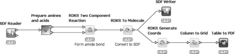
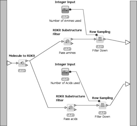
First, an SD file containing several amines and acids (in any order) is read in. Next, a meta-node encapsulates some preprocessing of the workflow. Specifically, it splits the input file into amines and acids and also reduces their number based on the user selection (e.g. three amines and three acids). Each group is then output to one of the two ports and passed to the Two Component Reaction node. This node simulates pairwise reactions between all molecules from both input ports and outputs a table with the resulting products. As the products are stored in the internal RDKit format, they need to be converted back to SDF before they can be written into a file (upper branch). A PDF file containing 2D depictions of all products is created in the lower branch. In the process, 2D coordinates are generated first and then the column with the 2D depictions is transformed into a grid. This means that all cells in the selected columns are arranged in a data table with, for example, four columns and as many rows as necessary to show all the products. A PDF is subsequently created from this table using the Table to PDF node, which is available on the KNIME Update Site as an extension.
The content of the meta-node that creates two sets of reactants is shown in Figure 6.10. First, the table containing the SDF records is processed with the Molecule to RDKit node, which converts the molecules into an internal format. Subsequently the converted molecules are passed to two Substructure Filter nodes that filter the molecules based on a SMARTS pattern. In the upper branch only amines pass the filter (SMARTS pattern [NX3;H2,Hl;!$(NC = O)] ), whereas in the lower branch only acids can pass through (SMARTS pattern [CX3](= O)[OX2Hl]). Both molecule sets are then passed through a Row Sampling node. Usually, the user can enter several parameters for sampling (e.g. the number of rows to pass through, if random or stratified sampling should be performed, or if only the top-n rows should be passed). However, in this case some of the parameters for the node are passed from a different node. The Integer Input node is part of a collection of so-called quickform nodes that allow injection of certain variables into a workflow from the outside. In the quickform node a description and a default value for the variable is entered, for example the number of amines/acids that should be passed through. When used inside a meta-node all variables defined by quickform nodes are exposed in the dialog of the meta-node, that is the user can configure the meta-node from the outside without opening it. Once values for each variable are available, they are passed into the row sampling nodes via special variable ports (red balls instead of the usual white triangles for data tables). In the sampling nodes' dialog the parameter for the number of rows is subsequently linked to the variable instead of taking the (default) value that was directly entered in the dialog.
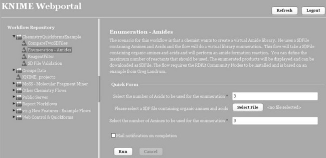
In combination with the commercial KNIME Server, quickform nodes can also be used outside meta-nodes. Here, variables are exposed in a web interface allowing the user to easily configure a workflow from a web browser and execute the workflow on the server, see Figure 6.11. The results (files, numbers,…) are also available via the browser. This concept allows 'power users' to build elaborate workflows and expose only certain parameters to the outside. Once uploaded to the server (directly from within KNIME), the 'normal' users can access the workflows via the web portal with the browser, provide input files and parameters, execute it on the server, and finally retrieve the results. A workflow can even be executed several times and all results are stored.
6.4.3 Classifying cell images
The third example workflow solves a common task in bioinformatics: the automated classification of cell images. One use case is the treatment of cells with different substances at various concentrations. At some point cells start to die and the task is to ascertain the lethal concentration automatically. For this, cell cultures are grown in 96-well plates and are treated with the substances in different concentrations. On each plate there are always positive and negative controls, for example the cell cultures without additional substances and cultures with very high concentrations of known activity, respectively.
Automated imaging systems take pictures, one for each well. Using the Image Processing nodes (which again rely on the free Imglib [6]), which are also available from the community contributions, these images can be analyzed. As this workflow is again quite complex, we show the outline in Figure 6.12.
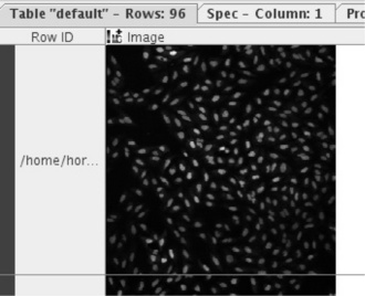
In the first step, Image Readers are used to load all images from a directory into KNIME. The Image Processing feature comes with a new data type for images to enable them to be used in data tables in the same way as strings, numbers, or molecules. Figure 6.13 shows one such image in KNIME's table view (the images are taken from the public SBS Bioimage CNT dataset).
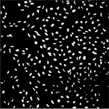
As there are two sets of images, one for the nuclei and one for the cytoplasm, before the features are computed they are combined into one table. The image features are computed independently for each single cell. Therefore the cells have to be identified first. This is performed by taking the nuclei images and applying a binary thresholder to distinguish the nuclei clearly from the background, see Figure 6.14.
These images are subsequently used as seeds for a so-called Voronoi segmentation. This process takes the cytoplasm images and segments them into many different non-overlapping regions around the seeds.
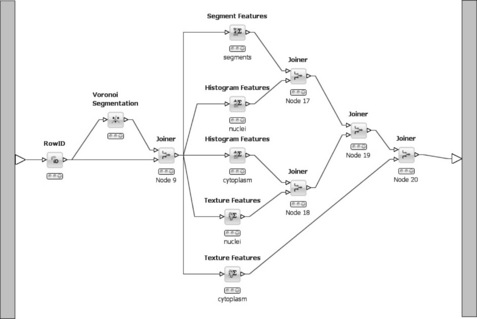
These segments are used to compute a variety of features such as histogram-based, texture-based, or segment-based features. The workflow part that deals with segmentation and feature generation is shown in Figure 6.15. As KNIME makes use of multicore systems and executes independent branches of a workflow in parallel, the workflow layout shown in the figure ensures that all features are computed in parallel. In the end they need to be re-combined into a single table using a cascade of Joiner nodes.
The computed features are all numeric or nominal, with the result that the remaining parts of the workflow – building a predictive model and applying it to unclassified images – are straightforward (and therefore not shown here; a similar example is given in Figure 6.1). All features originating from the control samples are used to build the model, that is a decision tree and all other segments are subsequently classified using this model.
6.4.4 Next Generation Sequencing
The workflow described here (Figure 6.16) is an example of how to use KNIME for Next Generation Sequencing (NGS) data analysis [7]. In particular, it describes typical parts of a data analysis workflow with regard to RNA-sequencing, DNA-sequencing, and ChlP-sequencing. It does not try to show a complete or perfect workflow but rather to point out some of the features of what can be done and explicit NGS relevant tools that can be used. This and similar workflows are used by Institute Pasteur.
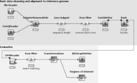
In general, this workflow reads-in FastQ formatted data, which is cleaned and filtered, then aligned to a reference genome (hg19) using bowtie [8] (upper part). The results are read and filtered and then written into a BEDGraph [9] file for visualization using, for example, GBrowse [10] or UCSC [11] genome browser (lower part). Regions of interest are also being identified.
As this workflow is also quite complex, we only highlight the most interesting parts. A complete description of an even more elaborate workflow is available in a separate publication [7]. Similar to the previous workflows, this one also makes use of the KNIME Community Contributions. The NGS package offers special nodes for dealing with NGS-related data. One example is the FastQ Reader, which reads the de facto standard FastQ file format using the BioJava library. Its output is a data table containing the cluster ID and the sequence along with the quality information. The File Reader reads parameters for the subsequent Adapter Removal Adv node, such as adapter sequences or other contaminating sequences, similarity threshold, quality threshold, and minimum overlap. This latter node compares each sequence from the FastQ file (target) with all sequences from the parameter file (query) and removes contaminations. The output is the second input table with adapters removed from the input sequences. The following nodes compute the sequence length and filter out very short sequences before writing everything back into a FastQ file. The subsequent 'Bash' node is only connected to its predecessor with a variable port. This ensures that it is not executed before the FastQ file has been written. The node executes a bash-script, which calls the bowtie program to align all sequences to the reference genome (hg19). Its output is a SAM formatted file with the information from the alignment. This is read in with the SAM Reader (again connected with a variable port to its predecessor). The next nodes select only sequences that align to the reference genome (Row Filter) and apply various transformations that result in a data table holding the original sequences, the chromosomes from the reference genomes and the positions in the sequences where there has been a mismatch in the alignment process (Meta Node). This information is subsequently written out into a BEDGraph file.
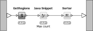
In the second branch, the ROI meta-node (see Figure 6.17) extracts the regions of interest (i.e. consecutive regions of coverage between the sequences and the reference chromosome). This is especially interesting when analyzing small RNA. The input is a list of positions from the reference genome with associated coverage. This list is already sorted by chromosome and position. The GetRegions node identifies regions of interest (ROIs). A ROI is defined as having entries in the input table with the same chromosome name and increasing (by one) positions, that is consecutive regions of coverage. Values are stored in a string column and concatenated using a space as a separator. Next, a Java Snippet retrieves the maximum count value from the count string whereupon all rows are sorted by that value to retrieve the regions with the highest coverage as the top entries in the output table.
Further open source tools for genomic data analysis are described in Chapter 8 by Tsirigos and co-authors.
6.5 Conclusion and outlook
It is possible to perform sophisticated data analysis tasks in KNIME using completely free software. The many contributors from the KNIME community ensure that the number of freely available extensions will continue to grow in the future, providing even more application areas in which KNIME can be used at no cost. There are, naturally, some areas in which no free methods are available and situations where guaranteed support is necessary when reliability is crucial for the success of projects. This is where commercial vendors come into play. KNIME's modularity and licensing model facilitates the usage of a mixture of free and non-free components. Another important aspect is the existence of the KNIME.com company which not only sells training courses, provides professional support, and develops enterprise extensions but also plays a key role in the further development of KNIME's free open source core.
6.6 Acknowledgments
We would like to thank the authors of the extensions described here for making their nodes available to KNIME. Special acknowledgments also go to Greg Landrum, Dmitry Pavlov, Frank Schaffer, and Martin Horn for providing some of the example workflows shown in this chapter.
6.7 References
[1] KNIME. http://www.knime.org/. Accessed 18 August 2011.
[2] KNIME.com. http://www.knime.com/products. Accessed 18 August 2011.
[3] KNIME Community Contributions. http://tech.knime.org/community. Accessed 18 August 2011.
[4] GGA Software Services LLC. Indigo. http://ggasoftware.com/opensource/ indigo. Accessed 18 August 2011.
[5] RDKit. http://www.rdkit.org/. Accessed 18 August 2011.
[6] Imglib. http://pacific.mpi-cbg.de/wiki/index.php/Imglib. Accessed 18 August 2011.
[7] Jagla, B., Wiswesdel, B., Coppee, J.Y. Extending KNIME for Next Generation Sequencing data analysis. Bioinformatics. 2011; 20:2907–2909.
[8] Langmead B, Trapnell C, Pop M, Salzberg SL. Ultrafast and memory-efficient alignment of short DNA sequences to the human genome. Genome Biol 10:R25.
[9] BEDGraph. http://genome.ucsc.edu/goldenPath/help/bedgraph.html. Accessed 17 August 2011.
[10] Gbrowse. http://gmod.org/wiki/GBrowse. Accessed 27 December 2011.
[11] Kent, W.J., et al. The human genome browser at UCSC. Genome Res. 2002; 12(6):996–1006.