
GenomicTools: an open source platform for developing high-throughput analytics in genomics
Abstract:
Following the dramatic reduction of sequencing cost, research laboratories have been producing huge amounts of data, measuring DNA variations, RNA abundances, protein–DNA interactions, DNA methylation levels, and even chromosomal conformations. Making sense of terabytes of data requires reliable data management, computational resources, and, eventually, efficient computational methods for pre-processing, quality control, analysis and meta-analysis. In this work, we present a flexible computational platform for facilitating the development of pipelines to accomplish such computational tasks. For example, the user can easily create average read profiles across transcriptional start sites or enhancer sites, quickly prototype customized peak discovery methods for ChIP-seq experiments, perform genome-wide statistical tests such as enrichment analyses, and design controls via user-designed randomization schemes, among other applications.
8.1 Introduction
The advent of high-throughput sequencing techniques initiated by pyrosequencing in 2004 [1] is expected to accelerate the pace of discovery in life sciences. Indeed, the rapidly and inexpensively produced super-exponential amount of data (e.g. short sequence patterns referred to as reads) from various high-throughput sequencing platforms allows the scientific community to study specific biological problems in depth, such as quantification of alternative splicing in tissues [2, 3], human disease [4], discovery of new fusion genes in cancer [5, 6], improvement of genome assembly [7], and transcript identification [8–11].
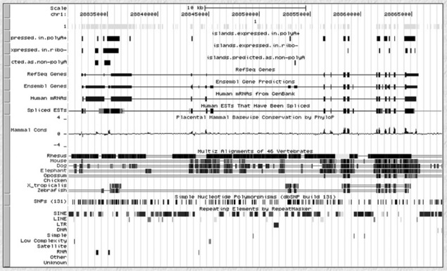
The common steps in many high-throughput sequencing studies include: (1) alignment of reads directly to a reference transcriptome or genome ('read mapping'), (2) identification of expressed genes, isoforms or binding sites; and (3) differential analysis across samples. An in-depth review of standard steps in RNA-seq and ChlP-seq computational pipelines is published by Pepke and colleagues [12]. It is worth pointing out that genome-wide data, such as transcripts/genes, exons/introns, promoter sites, sequences, multiple sequence alignments, transcription factor binding sites, intergenic regions, repeat elements, microarray probes (expression, SNP, CNV, etc.), sequencing data (RNA-seq, ChlP-seq, DNA-seq, etc.), chromosomal conformations (3C-seq, 4C-seq, etc.), and inter-chromosomal associations can easily be represented as sets of genomic intervals (see Figure 8.1).
Given the huge volume of available data, new efficient computational tools are required in order to efficiently perform analysis tasks such as those outlined above [13]. Currently, freely available computational tools for large-scale data analytics include Bioconductor [14], Galaxy [15], Genomic Regions Enrichment of Annotations Tool (GREAT) [16], USCS genome browser [17] and Integrated Genome Browser (IGB) [18]. For the readers' convenience, we report here the fundamental aspects of each tool. Bioconductor uses the R statistical programming framework to provide tools for the analysis and comprehension of high-throughput genomic data. The functional scope of Bioconductor packages includes the analysis of DNA microarray, sequence, flow, and SNP data. Galaxy is an open web-based platform for genomic research, based around reusable analysis templates that users can manipulate and run repeatedly on different data sets. Galaxy has been used for different types of genomic research, for example investigations of epigenetics, chromatin profiling, transcriptional enhancers, and genome-environment interactions. GREAT is available as a web application that was designed to analyze the functional significance of cis-regulatory regions identified by localized measurements of DNA binding events across an entire genome. The USCS genome browser and IGB are web-based visualization platforms that incorporate data from several public databases.
Despite the existence of these sophisticated tools for genome analysis, they are not designed to efficiently process multiple large data sets–such as the ones obtained from high-throughput sequencing–and suffer from poor memory management as essentially all data needs to be loaded into memory and/or sent over the network.
In an attempt to address some of these issues, Quinlan and Hall have developed the BEDTools suite [19]. We predict that the BEDTools initiative will lead into a competition for a new set of tools focused on processing genomic data as streams. This new set of tools will provide the means to efficiently handle large genomic data sets, thus providing a computational platform that facilitates the development of bioinformatics applications. These tools may then be integrated with or incorporated into other bioinformatics tools/environments, including those mentioned above.
The motivation behind GenomicTools (first presented in [20] as an 'applications note') was to create a computational platform for developing customized analytics for genomic data sets with minimal memory and intermediate file requirements in order to address the bottleneck caused by the increasing influx of genome-wide data sets. GenomicTools is available both as command-line tools for building applications in a UNIX-like environment and as documented C++ classes for further development. The open source aspect of GenomicTools is important as it allows users to easily incorporate their own analysis methods with the published tools and to modify the tools to suit their specific data analysis needs. Although similar in motivation to BEDTools, it is in several aspects more general than BEDTools and it addresses several issues that BEDTools do not adequately address. We summarize the novelty of GenomicTools below.
![]() Novel operations; in GenomicTools the focus is not simply on overlap computations as in BEDTools. GenomicTools is designed to perform a variety of simple mathematical operations on set genomic intervals (as a pre-processing step) and then a variety of complex operations can be performed, such as overlap, offset or scanning computations (Figure 8.2), that is a superset of the operations offered by BEDTools.
Novel operations; in GenomicTools the focus is not simply on overlap computations as in BEDTools. GenomicTools is designed to perform a variety of simple mathematical operations on set genomic intervals (as a pre-processing step) and then a variety of complex operations can be performed, such as overlap, offset or scanning computations (Figure 8.2), that is a superset of the operations offered by BEDTools.
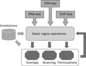
Figure 8.2 Flow-chart describing the various functionalities of the GenomicTools suite: basic region operations are implemented in genomic_regions whereas complex operations are implemented in genomic_overlaps, genomic_scans and permutation_test (source: adapted figure 1 from Tsirigos et al. [20])
![]() Relaxed data set restrictions: GenomicTools allows several of its operations to operate on sets of genomic regions rather than sets of single genomic intervals as in BEDTools, for example it makes full use of all 'exons' in BED entries. BEDTools operates on single-'exon' BED entries.
Relaxed data set restrictions: GenomicTools allows several of its operations to operate on sets of genomic regions rather than sets of single genomic intervals as in BEDTools, for example it makes full use of all 'exons' in BED entries. BEDTools operates on single-'exon' BED entries.
![]() Full stream-computing design: in GenomicTools no files are loaded into memory but are processed instead as streams: this minimizes memory requirements and allows the simultaneous processing of several files (e.g. different replicates, patient samples, etc.).
Full stream-computing design: in GenomicTools no files are loaded into memory but are processed instead as streams: this minimizes memory requirements and allows the simultaneous processing of several files (e.g. different replicates, patient samples, etc.).
![]() C++ API: GenomicTools command-line operations are implemented as C++ class methods in a convenient API, which may be used by developers to write new applications entirely in C++, for example novel peak finders.
C++ API: GenomicTools command-line operations are implemented as C++ class methods in a convenient API, which may be used by developers to write new applications entirely in C++, for example novel peak finders.
![]() Auxiliary tools: GenomicTools offers a set of auxiliary command-line tools (permutation_test, vectors, and matrix) to facilitate the construction of command-line pipelines as they implement basic mathematical and statistical operations on vectors and matrices.
Auxiliary tools: GenomicTools offers a set of auxiliary command-line tools (permutation_test, vectors, and matrix) to facilitate the construction of command-line pipelines as they implement basic mathematical and statistical operations on vectors and matrices.
![]() Performance: GenomicTools improves performance over BEDTools both in terms of time and memory requirements.
Performance: GenomicTools improves performance over BEDTools both in terms of time and memory requirements.
Research institutions as well industry sectors in life sciences, such as pharmaceutical and medical research companies, that make extensive use of high-throughput sequencing technologies, are expected to use these tools. Naturally, these tools can also be used for different kinds of genomics studies, and were in fact initially developed for this reason. More specifically, our computational genomics group at IBM Research has used an early version of this tool–before it was released to the public–for computational studies of repeat elements in mammalian genomes [21, 22], analysis of gene expression tiling array data in Drosophila [23], and the study of dynamic changes in human DNA methylation during differentiation [24].
The rest of this chapter presents the GenomicTools platform (version 2.0, released in September 2011) and is organized as follows. The following section provides the necessary definitions as well as fundamental information on the input file formats used in GenomicTools. There is then an overview of the tools, followed by a more in-depth presentation of some aspects of the C++ implementation. Several practical examples are given using GenomicTools for computational genomics analyses in the context of a simple ChIP-seq pipeline case study. Finally, a comparison of the performance of GenomicTools against BEDTools and Bioconductor is provided.
8.2 Data types
In this section, we will introduce the basic definitions of a genomic interval and genomic regions. We will also describe the input file formats supported by GenomicTools.
8.2.1 Definitions
A genomic interval is a tuple: < chromosome, strand, start position, end position > .
A genomic region is an ordered set of genomic intervals. Note that this is a rather broad definition, which allows for the inclusion of genomic intervals from different chromosomes and/or strands, as well as intervals that overlap. In GenomicTools, this definition of genomic regions is implemented in the REG file format, which we introduce in the next section.
Genomic regions are characterized by several properties. A genomic region is compatible if and only if all its intervals are in the same chromosome and (optionally) strand. A genomic region is sorted if and only if its intervals are sorted first by chromosome, then optionally by strand and finally by start position. A genomic region is non-overlapping if and only if its intervals are non-overlapping in all pair-wise combinations. A genomic region is a single-interval region if and only if it contains exactly one interval. Operations on genomic regions may require that certain properties be satisfied before they can be successfully executed.
A genomic region set is an ordered set of genomic regions. A genomic region set is sorted if and only if its regions are single-interval regions and they appear in the sort order described above. As before, operations on genomic region sets may require that certain properties be satisfied before they can be successfully executed.
In GenomicTools, all input files contain a single genomic region set as defined above. Every line of these files corresponds to a single genomic region possibly annotated with additional information, such as labels, depending on the particular file format (see next section).
8.2.2 Supported file formats
The GenomicTools platform supports the standard BED [25], GFF [26], and SAM [27] file formats. Input files can also be converted into WIG format [28]. Additionally, we propose a new simple format, the REG format, as an attempt to distill the minimum common information from the BED/GFF/SAM formats while allowing for the more general definition of a genomic region as defined above. Each line in a REG file represents a labeled genomic region, where the label is separated from the genomic region via a < TAB > character. A simple REG file representing a set of RNA-seq reads is shown below.
Another example is the following REG file carrying information on gene exons (note that every line is a set of genomic intervals).
Note that this format is a generalization of the BED format because it allows overlapping intervals within a given region (Gene#1 in the above example). This is particularly useful when we need to group exons of a set of transcript isoforms of the same gene. Additionally, it allows intervals from different chromosomes and strands to be grouped in each line, and this helps represent gene fusions and interchromosomal associations.
In terms of C++ implementation, each genomic region (i.e. each line in an input file) is stored as an instance of the GenomicRegion class or its derived classes for BED, GFF, and SAM formats (see C++ API for developers for details). The entire file is stored as an instance of the GenomicRegionSet class, although not necessarily fully loaded in memory.
8.3 Tools overview
The GenomicTools platform is built on top of the genomic_intervals C++ library described in the next section. Its functions are bundled in four command-line tools: (1) genomic_regions, for basic genomic regions operations; (2) genomic_overlaps for comparing sets of regions and computing offsets; (3) genomic_scans for window-based operations; and (4) permutation_test for enrichment analyses. Additionally, in this distribution, we are including auxiliary tools for manipulating vectors and matrices.
The flow-chart in Figure 8.2 summarizes the role of each of the command-line tools in our pipeline model. Briefly, the pipeline inputs in REG/GFF/BED/SAM format represent either sequenced read alignments (e.g. from DNA-seq, RNA-seq, ChIP-seq experiments) or annotations from public databases. The annotations that can be utilized in our pipeline fall into two categories: (1) genomic annotations represented as genomic regions, such as the known genes set in the UCSC Genome Browser; and (2) functional annotations, for example from Gene Ontology [29]. Computations are performed in two levels: (1) basic interval operations (such as unions, intersections, shifting, flanking, etc.) are implemented by the genomic_regions command-line tool; and (2) complex operations (overlaps, offsets, scanning and permutations) implemented by the genomic_overlaps, genomic_scans and permutation_ test command-line tools take as input the regions that have undergone basic processing and produce results. Basic and complex operations can be combined into fairly elaborate scripts that can address a wide range of issues during the course of a bioinformatics project.
In large-scale analyses it is important to avoid biases introduced by the complexity and redundancy of large genome-wide data sets. For example, when computing an average gene TSS profile for ChIP-seq reads, it is important to create a 'non-redundant' set of gene TSSs, which is not a trivial task because gene transcripts with different identifiers and possibly originating in different databases may report slightly different TSSs for transcripts that are in fact the same. The operations implemented in the GenomicTools platform can help correct for these biases as a preprocessing step before the actual computation takes place, or assess the effect of the bias on the result.
8.3.1 The genomic_regions tool
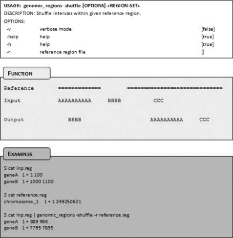
The genomic_regions tool is designed to perform basic operations on genomic region files. These are: (1) line-based operations, such as shifting, shuffling, sorting, and modifying genomic regions; and (2) file-based operations such as inverting or linking genomic regions. Table 8.1 comprises the complete list of operations and each operation is documented in the user's manual, an entry of which is shown in Figure 8.3. To get a list of options without the need to refer to the manual, simply use the '-h' option.
Table 8.1
Summary of operations of the genomic_regions tool
| Operation | Description |
| align | Aligns sequences to reference genome (line-based) |
| bed | Converts input regions to BED format (line-based) |
| bounds | Checks interval against chromosome bounds and removes invalid intervals (line-based) |
| center | Prints center interval (line-based) |
| connect | Connects intervals from minimum start to maximum stop (line-based) |
| diff | Computes the difference between successive intervals (line-based) |
| dist | Computes distances between successive intervals (line-based) |
| divide | Divides intervals in the middle (line-based) |
| fix | Removes invalid intervals, i.e. start < 1 or start > stop (line-based) |
| gdist | Computes distances of successive regions (file-based) |
| int | Computes the intersection of input intervals (line-based) |
| inv | Inverts regions given the genome chromosomal boundaries (file-based) |
| link | Links consecutive regions to produce a non-overlapping set (file-based) |
| n | Computes total interval length, including possible overlaps (line-based) |
| pos | Modifies interval start/stop positions (line-based) |
| reg | Converts to REG format (line-based) |
| rnd | Randomizes region across entire genome (line-based) |
| select | Selects a subset of intervals according to their relative start positions (line-based) |
| shift | Shifts interval start/stop positions (line-based) |
| shiftp | Shifts interval 5'/3' positions (line-based) |
| shuffl | Shuffles intervals within given reference region (line-based) |
| sort | Sorts intervals (line-based) |
| split | Splits regions into their intervals which are printed on separate lines (line-based) |
| strand | Modifies interval strand information (line-based) |
| test | Tests whether genomic regions are sorted and nonoverlapping (file-based) |
| union | Computes the interval union (line-based) |
| wig | Converts to UCSC wiggle format (line-based) |
| win | Creates new intervals by sliding windows (line-based) |
| x | Extracts corresponding sequences from DNA (line-based) |
8.3.2 The genomic_overlaps tool
The genomic_overlaps tool allows the user to compute various measures of overlaps between sets of regions (see online documentation for the complete list of operations). This is achieved by providing a set of densities of matched regions; and (4) computing overlap offsets. Applications include computation of gene expression from RNA-seq data (e.g. RPKMs [30]), construction of average read profiles or heatmaps across transcriptional start sites (TSSs), enrichment analyses of virtually any genomic data set, such as genes of specific functional categories, repeat types, single nucleotide polymorphisms (SNPs), or cancer-associated regions.
Table 8.2
Summary of usage and operations of the genomic_overlaps tool
| Operation | Description |
| count | Counts the number of overlapping test regions per reference region |
| coverage | Calculates the depth coverage (i.e. the total number of overlapping nucleotides) per reference region |
| density | Computes the density (i.e. the coverage divided by the size of the reference region) of overlaps per reference region |
| intersect | Computes the intersection between all pairs of test and reference regions |
| offset | Computes the distances of test regions from their overlapping reference regions |
| overlap | Finds the overlaps between all pairs of test and reference regions |
| subset | Picks a subset of test regions depending on their overlap with reference regions |
8.3.3 The genomic_scans tool
The genomic_scans tool can be used for window-based computations such as peak discovery. The command-line version offers several parameters for controlling the window size, statistical tests, etc. Users with basic C/C++ skills can easily modify the source code to perform the statistical test of their choice using the GenomicRegionSetScanner class described below.
8.3.4 The permutation_test tool
This tool executes row permutations to determine p-values and q-values for all the categories contained in the input file given the statistic chosen by the user (see Table 8.4 for available statistical tests). More specifically, the statistic on the set of rows annotated by a given category is compared against the same statistic on permuted versions of the input on the value column. For an example, see Identifying enriched Gene Ontology terms.
Table 8.4
Supported statistics for the permutation tests
| Statistic | Description |
| sum | The sum of values in a given category |
| n | Number of values > 0 |
| sens | Sensitivity |
| spec | Specificity |
| ratio | Mean of values divided by mean of values in the background |
| t | t-test between mean of values against mean of values in the background |
8.3.5 Vector and matrix operations
The GenomicTools distribution includes two command-line tools for manipulating labeled vectors and matrices. The input format for the vectors command-line tool is a series of lines, each of which has two TAB-separated fields (label and SPACE-separated vector elements). The label field is optional. Similarly, the input format of the matrix command-line tool is an optional header containing column labels followed by a series of labeled vectors (defined above) of the same number of elements. The full list of supported vector and matrix operations can be found in the User's Manual online (see section 8.8).
8.4 C++ API for developers
Users with basic C++ skills can make use of the genomic_intervals library, particularly for window-based computations and overlaps. All implemented classes are fully documented using Doxygen [31] (see Figure 8.4 for a snapshot). Access to full documentation is provided along with the source code distribution. In the following sections, we describe the main classes that are used to represent the genomic data and perform the various operations.
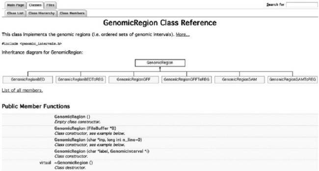
Figure 8.4 Example entry (partial) from the C++ API documentation produced using Doxygen and available online with the source code distribution
8.4.1 The GenomicInterval and GenomicRegion classes
The GenomicInterval class implements the notion of a genomic interval, that is an interval annotated with chromosome and strand information. The GenomicRegion class implements the notion of a genomic region (in REG format), that is a labeled ordered set of genomic intervals, and corresponds to one single line in the input file. The genomic intervals are stored as C++ STL vectors, but there is also an option of C++ STL lists for developers. This class has a series of constructors, which create genomic regions from an input file (accessed via the FileBuffer class), or from a character array. The methods of this class are classified into four categories:
![]() read & print methods: read and print genomic intervals in various formats;
read & print methods: read and print genomic intervals in various formats;
![]() get & set methods: retrieve and set class variables, such as label, chromosome, etc.;
get & set methods: retrieve and set class variables, such as label, chromosome, etc.;
![]() check & compare methods: obtain information about region properties (sorted, compatible, etc.), and their relationship with other regions (overlaps, order, etc.);
check & compare methods: obtain information about region properties (sorted, compatible, etc.), and their relationship with other regions (overlaps, order, etc.);
![]() operations: execute operations between or within regions, such as union, difference, etc.
operations: execute operations between or within regions, such as union, difference, etc.
This GenomicRegion class contains just enough information for the minimal requirements of the REG format. Most methods described above are implemented as virtual so as to allow for class extensions, which provide full support for:
The virtual methods are redefined–when necessary–for each derived class in order to properly read, print, and update the extra variables of each format.
Additionally, for each format, we provide simple classes whose goal is to only read in the corresponding format and immediately convert it into the REG format. These classes are used when the extra variables of the input format are not needed for a particular computation, and can save both time and memory resources. These classes are:
8.4.2 The GenomicRegionSet class
The GenomicRegionSet class implements the notion of a set of genomic regions that corresponds to an entire input file, for example the set of known genes, or aligned reads from a sequencing experiment. The main data element stored in this class is an array of instances of the GenomicRegion class (or any of its derived classes). The input file can be read from the standard input to facilitate pipelined execution, and is not necessarily loaded fully in memory in order to minimize memory requirements: essentially, the input files are read and processed sequentially one line at a time, and the data for each line are discarded when no longer needed for the particular computation. In the next section we show an example of allocating an instance of this class. The operations of the genomic_regions command-line tool summarized in Table 8.1 are implemented as methods in this class (see the User's Manual for details).
8.4.3 The GenomicRegionSetScanner class
This class helps scan by sliding windows an instance of GenomicRegionSet and is used by the genomic_scans command-line tool. The main advantage of this implementation of sliding window computations is that it is done sequentially without the need of storing the entire input intervals in memory. A practical use of this class is to develop customized window-based peak discovery algorithms. As shown in the example below, this class can be used to determine the number of reads in signal and control region sets in sliding windows along the entire genome.
8.4.4 The GenomicRegionSetOverlaps class and its extensions
This class is an abstract class used for determining and manipulating overlaps between two regions sets. It is extended into two classes. SortedGenomicRegionSetOverlaps is used on sorted region sets. The sort order is first by chromosome, then (optionally) by strand, and finally by start position. The algorithm used to compute overlaps in this class is a generalization of the standard merge-sort algorithm modified so as to handle intervals. As before, the main advantage of this implementation is that processing is done sequentially without the need of storing the entire input intervals in memory. The algorithm operates on sorted inputs, scans the files sequentially and computes all overlaps essentially using a merge-sort algorithm adapted to handle intervals. An intermediate buffer keeps all the overlaps of index regions with the current query, as they may also overlap with the next query.
UnsortedGenomicRegionSetOverlaps is used on unsorted region sets. The algorithm used here is a modification of the algorithm proposed by Kent et al. [17], where we allow the number of levels and the number of bins per level to be chosen arbitrarily.
The example below demonstrates the use of both derived classes (this is taken from the source code file 'genomic_overlaps.cpp').
8.5 Case study: a simple ChIP-seq pipeline
In this chapter, we demonstrate the utility of GenomicTools in constructing a simple pipeline for ChIP-seq analysis. The pipeline helps accomplish the following tasks: (1) produce data for popular plots such as read profiles and read density heatmaps; (2) create genome browser tracks for visualization; (3) identify peaks as potential binding sites; and (4) perform an enrichment analysis. ChIP-seq studies are now widely used to elucidate the molecular function of the cell under normal conditions as well as under stress or disease (see for example [32–34]). As they reveal the genomic positions of protein interactions, such as transcription factors and histone modification, with DNA, they can help create networks of interactions and reveal undiscovered biological mechanisms. Our tools help set up computational pipelines that drive this discovery. The following examples use UNIX command-line functions, but they also run on Cygwin under MS Windows.
8.5.1 Creating ChIP-seq read profiles
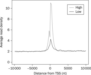
ChIP-seq read profiles are heavily used in ChIP-seq studies because they offer an easy method for data validation regarding the relative position of the ChIP-seq peaks (i.e. potential binding sites) with respect to chosen genomic features, such as gene transcriptional start sites (TSSs) or binding sites of other factors, such as enhancers. Additional validation is possible if expression data are available and the transcription factor or histone modification mark under ChIP-seq investigation is activating or repressive. In such a case, its read profile can be computed separately for genes of high versus low expression and its activating or repressive role confirmed.
Creating read profiles using GenomicTools is straightforward, as demonstrated in the following example. First, the user creates the TSS regions using as input the gene transcript chromosomal coordinates in 'genes.bed', which can be downloaded, for example, from the UCSC Genome Browser web site. This is done using the genomic_regions tool 'pos' and 'shift' operations: the former chooses the 5' end of gene transcripts (i.e. the TSS) and the latter performs a 10 kb flanking operation upstream and downstream of the TSS.
chr1 3044313 3044814 ENSMUSG00000090025:ENSMUST00000160944 1000 +
chr1 3092096 3092206 ENSMUSG00000064842:ENSMUST00000082908 1000 +
chr1 3456667 3503634 ENSMUSG00000089699:ENSMUST00000161581 1000 +
chr1 3670235 3671871 ENSMUSG00000073742:ENSMUST00000097833 1000 +
$ cat genes.bed ![]() genomic_regions pos -op 5p
genomic_regions pos -op 5p ![]() genomic_regions shiftp-5p -10000 -3p + 10000 > TSS.10 kb.bed
genomic_regions shiftp-5p -10000 -3p + 10000 > TSS.10 kb.bed
chr1 3034313 3054314 ENSMUSG00000090025:ENSMUST00000160944 1000 +
chr1 3082096 3102097 ENSMUSG00000064842:ENSMUST00000082908 1000 +
chr1 3446667 3466668 ENSMUSG00000089699:ENSMUST00000161581 1000 +
chr1 3660235 3680236 ENSMUSG00000073742:ENSMUST00000097833 1000 +
chr1 4509097 4529098 ENSMUSG00000064376:ENSMUST00000082442 1000 +
chr1 4787868 4807869 ENSMUSG00000025903:ENSMUST00000134384 1000 +
chr1 4787903 4807904 ENSMUSG00000025903:ENSMUST00000027036 1000 +
Next, the distances of the mapped ChlP-seq reads from the TSS regions are computed using the genomic_overlaps tool 'offset' operation. The 'offset' operation allows the user to choose a reference point for the query regions ('-op' option), and to express the computed offset as a fraction of the query region size ('-a' option) instead of an absolute number. Also, in this particular application, the strand information is ignored ('-i' option), because binding occurs both sense and anti-sense of the affected transcript.
Finally, the computed offsets can be separated in genes of high versus low expression, histogrammed using the vectors tool (operation 'hist') and plotted using R (see Figure 8.5 for a sample plot), Excel or any other similar tool or environment. For example, if the 'offset.txt' file computed above was separated into two files 'offset.high.txt' for the genes of high expression and 'offset.low.txt' for the genes of low expression, then:
Note that the histogram counts in column #3 need to be normalized by the number of genes in each group. Option '-n 6' sets the number of decimals to 6 and '-b 100' the number of histogram bins to 100.
8.5.2 Creating ChlP-seq read density heatmaps
Although average ChlP-seq profiles are useful for easy visualization and validation, they do not reveal the exact binding site position per gene. This can be achieved by ChlP-seq read density heatmaps around TSSs (Figure 8.6). To produce the data for this type of plot, the user can simply utilize the vectors operations '-merge' and '-bins', so that now the histograms are produced per gene rather than for the entire offset file.
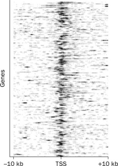
In the example above, we used a total of 200 bins (option '-b 200'), and a smoothing parameter '-m 10', which sums the results in each series of consecutive 10 bins.
8.5.3 Creating window-based read densities
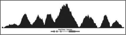
In ChIP-seq studies, researchers are interested in visualizing the densities of their ChIP-seq reads at a genome-wide scale so that they can understand the behavior of the studied protein in genes of interest. GenomicTools can be used to create window-based read densities to be displayed as a wiggle track in the UCSC Genome Browser (Figure 8.7). First, the user needs to decide on the window parameters: (1) the size of the window; (2) the distance between consecutive windows; and (3) minimum number of read allowed in each window. The last two parameters establish a tradeoff between resolution and output file size. Here are some typical values:
Then, the user needs to create a file describing the chromosomal bounds in REG or BED format:
The genomic_scans tool can be used to compute the counts of reads stored in 'chipseq.bed' in sliding windows across the genome. Finally, the center of each window is computed and the '-wig' operation of genomic_ regions converts to the wiggle format for display in the UCSC Genome Browser (Figure 8.7):
8.5.4 Identifying window-based peaks
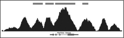
GenomicTools can also be used to identify window-based peaks and to display them as a BED track in the UCSC Genome Browser. This is achieved using the operation 'peaks' of the genomic_scans tool. As in the 'counts' operation in the example above, the user needs to determine the window size and distance as well as the minimum number of reads in the window. For each window, p-values are computed using the binomial probability. A p-value cutoff can be enforced using the '-pval' option. The user can specify a file containing control reads ('control.bed' in our example below). If no control reads are specified, the computed p-values are based on a random background. Finally, the 'bed' operation of the genomic_regions tool is used to convert the output to the BED format for visualization in the UCSC Genome browser (Figure 8.8, upper track):
8.5.5 Identifying enriched Gene Ontology terms
In a given biological context, for example a tissue type or disease state, certain proteins (transcription factors or modified histones) tend to bind to genes of specific functional categories. Gene enrichment analysis can identify these categories. In the GenomicTools platform, enrichment analysis is performed using the permutation_test tool, which performs row permutations of inputs comprising measurements and annotations (see below). Using the ChlP-seq peaks computed above, we first calculate their densities across gene TSS regions – flanked by 10 kb – using the 'density' operation of the genomic_overlaps tool:
Then, suppose we have a file containing gene annotations in a TAB-separated format where the first column is a gene id and the second column is a SPACE-separated list of annotations for the corresponding gene. The file must be sorted by gene id. For our example, we will use 'gene.go', which contains annotations from the Gene Ontology [29]:
As an input, permutation_test needs to take a file containing three TAB-separated fields: the first field is an id (e.g. gene id), the second field is a value (e.g. density) and the third field is a SPACE-separated list of annotations. We first group the results in 'tss.val' by gene using 'vector -merge', then choose the maximum density per gene across transcripts using 'vector-max', and finally perform a join operation with 'gene.go' (note that the delimiter used in the join operation specified by option '-t' must be a TAB, i.e. Control-V-I):
Now, we can run the permutation_test tool (for details about the tool's options the reader is referred to the User's Manual)
$ permutation_test -v -h -S n -a -p 10000 -q 0.05 tss.val + go > peaks.
$ head peaks.enriched.go.in.tss.txt
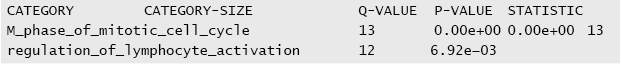
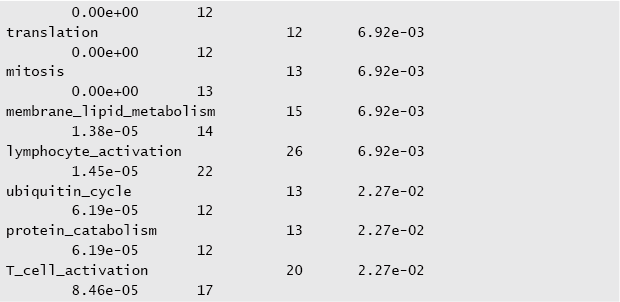
The output of the tool ranks each gene category according to the adjusted p-values (i.e. q-values) from the most to the least significant. In this particular scenario, where the input values correspond to binding sites in promoters as identified by our ChlP-seq analysis, the results of the enrichment analysis indicate that the assayed protein binds on genes that play a role in lymphocyte activation. This kind of analysis can be very powerful at generating novel biological hypothesis. Suppose that the assayed protein was never shown to participate in lymphocyte activation. Then, based on the evidence produced by the enrichment analysis above, biologists can design further experiments to prove (or reject) this hypothesis.
8.6 Performance
Typically, during the course of computational analyses of sequencing data, computational biologists experiment with different pre-processing and discovery algorithms. GenomicTools is designed to take advantage of sorted inputs (the sort order is chromosome → strand → start position) to create efficient pipelines that can handle numerous operations on multiple data sets repeated several times under different parameters. In the GenomicTools platform, the original data sets (e.g. the mapped reads in BED format) need to be sorted only once at the beginning of the project. As we show below, sorted inputs can lead to dramatic improvements in performance.
We evaluated the time and memory usage of GenomicTools and compared its performance to (1) the IRanges Bioconductor package [14]; and (2) the BEDTools suite [19]. The evaluation was run on a RHEL5/ x86-64bit platform with 12 GB of memory on the IBM Research Cloud.
For this evaluation we used sequenced reads obtained from the DREAM project [35], more specifically from challenge #1 of the DREAM6 competition. We downloaded the original FASTQ files (paired-end reads) representing mRNA-seq data from human embryonic stem cells from http://www.the-dream-project.org/challenges/dream6-alternative-splicing-challenge.
The FASTQ files were aligned to the reference human genome (version GRCh37, February 2009) using TopHat version 1.3.1 [36]. In total ~ 86 million reads were aligned and converted from BAM to BED format. In this evaluation, we measured how both CPU time and memory scale with increased input size. The task was to identify all pair-wise overlaps between a 'test' genomic interval file and a 'reference' genomic interval file. The former was obtained from the set of ~ 86 million sequenced reads using re-sampling without replacement (re-sampling of 1, 2, 4, 8, 16, 32 and 64 million reads), and the latter contained all annotated transcript exons from the ENSEMBL database [37], as well as all annotated repeat elements from the UCSC Genome Browser [17], that is a total of ~ 6.4 million entries.
As demonstrated in Figure 8.9, GenomicTools improves greatly on time performance (speed-up of up to ~ 3.8 compared to BEDTools and ~ 7.0 compared to the IRanges package of Bioconductor) if the inputs are sorted, and is therefore well suited for large-scale Bioinformatics projects. Additionally, GenomicTools makes virtually no use of memory, unlike IRanges and BEDTools, both of which use a significant amount of memory (Figure 8.10), thus limiting the number of such processes that can simultaneously run on the same system.
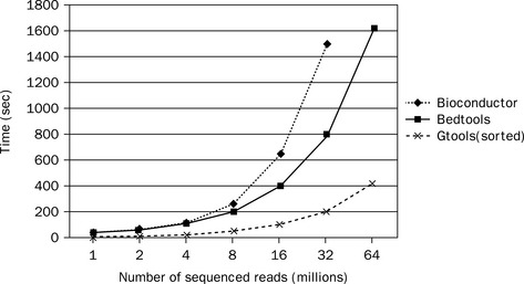
Figure 8.9 Time evaluation of the overlap operation between a set of sequenced reads of variable size (1 through 64 million reads in logarithmic scale) and a reference set comprising annotated exons and repeat elements (~ 6.4 million entries). Using GenomicTools on sorted input regions yields a speed-up of up to ~ 3.8 compared to BEDTools and ~ 7.0 compared to the IRanges package of Bioconductor
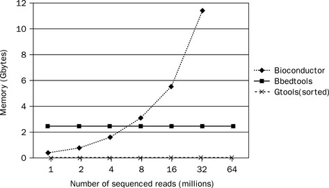
Figure 8.10 Memory evaluation of the overlap operation presented in Figure 8.10. Memory requirements for the IRanges package of Bioconductor increase with input size, which makes it impossible to handle big data sets (in this particular hardware setup of 12 GB memory we could only compute overlaps for up to 32 million reads). BEDTools uses a fixed amount of memory, which depends on the size of the reference input set (i.e. exons and repeat elements). GenomicTools uses no significant amount of memory, as all input files are read sequentially, but, of course, it has to rely on sorted inputs
8.7 Conclusion
It is becoming increasing apparent that humanity in general, and science in particular, can greatly benefit from properly applying the principles of openness, transparency, and sharing of information. The free open source initiatives in recent years have led to new interesting phenomena, such as crowd-sourcing, which bring together entire communities to everyone's benefit in some sort of collaborative competition. This notion of contribution was the single most significant motivation for making this suite of tools publicly and freely available. Soon after we decided to open source our software, we realized that it is one thing to use software internally, and a totally different thing to actually expose it to public usage. For example, we understood that for open source to be meaningful, the developer needs to undertake a variety of tasks, such as documenting the source code, creating a user's manual, tutorials, a web site, and also using some version control and a bug tracking system. Overall, we are convinced that this effort was worthwhile and that the open source trend is only going to get stronger in the next few years.
8.8 Resources
This chapter described version 2.0 of GenomicTools released in September 2011. The source code, documentation, user manual, example data sets and scripts are available online at http://code.google.com/p/ibm-cbc-genomic-tools/.
To install GenomicTools, follow these simple instructions:
There is a dependency on the GNU Scientific Library (GSL), which can be downloaded from http://www.gnu.org/software/gsl/.
Examples and associated input files and scripts are part of the source code distribution in the 'examples' subdirectory. The API documentation is stored in the 'doc' subdirectory.
For details about the options for each tool, the reader is referred to the User's Manual, which can be downloaded from http://code.google.com/p/ibm-cbc-genomic-tools/#Documentation.
For any questions, suggestions or comments contact Aristotelis Tsirigos at [email protected].
8.9 References
[1] Margulies, M., et al. Genome sequencing in microfabricated high-density picolitre reactors. Nature. 2005; 437(7057):376–380.
[2] Wang ET, et al., 'Alternative Isoform Regulation in Human Tissue Transcriptomes', Nature, Nature ;456(7221), 470–6.
[3] Blekhman, R., Marioni, J.C., Zumbo, P., Stephens, M., Gilad, Y. Sex-specific and lineage-specific alternative splicing in primates. Genome Research. 2010; 20(2):180–189.
[4] Wilhelm, B.T., et al. RNA-seq analysis of 2 closely related leukemia clones that differ in their self-renewal capacity. Blood. 2011; 117(2):e27–e38.
[5] Berger, M.F., et al. Integrative analysis of the melanoma transcriptome. Genome Research. 2010; 20(4):413–427.
[6] Maher, C.A., et al. Transcriptome Sequencing to Detect Gene Fusions in Cancer. Nature. 2009; 458(7234):97–101.
[7] Mortazavi, A., et al. Scaffolding a Caenorhabditis nematode genome with RNA-seq. Genome Research. 2010; 20(12):1740–1747.
[8] Denoeud, F., et al. Annotating genomes with massive-scale RNA sequencing. Denoeud F. 2008; 9(12):R175.
[9] Yassour, M., et al. Ab initio construction of a eukaryotic transcriptome by massively parallel mRNA sequencing. Proceedings of the National Academy of Sciences of the United States of America. 2009; 106(9):3264–3569.
[10] Guttman, M., et al. Ab initio reconstruction of cell type-specific transcriptomes in mouse reveals the conserved multi-exonic structure of lincRNAs. Nature Biotechnology. 2010; 28(5):503–510.
[11] Trapnell, C., et al. Transcript assembly and quantification by RNA-Seq reveals unannotated transcripts and isoform switching during cell differentiation. Nature Biotechnology. 2010; 28(5):511–515.
[12] Pepke, S., Wold, B., Mortazavi, A. Computation for ChlP-seq and RNA-seq studies. Nature Methods. 2009; 6(11):S22–S32.
[13] Garber, M., Grabherr, M.G., Guttman, M., Trapnell, C. Computational methods for transcriptome annotation and quantification using RNA-seq. Nature Methods. 2011; 8(6):469–477.
[14] Gentleman, R.C., et al. Bioconductor: open software development for computational biology and bioinformatics. Genome Biology. 2004; 5(10):R80.
[15] Goecks, J., Nekrutenko, A., Taylor, J. Galaxy: a comprehensive approach for supporting accessible, reproducible, and transparent computational research in the life sciences. Genome Biology. 2010; 11(8):R86.
[16] McLean, C.Y., et al. GREAT improves functional interpretation of cis-regulatory regions. Nature Biotechnology. 2010; 28(5):495–501.
[17] Kent, W.J., et al. The human genome browser at UCSC. Genome Research. 2002; 12(6):996–1006.
[18] Nicol, J.W., Helt, G.A., Blanchard, S.G., Jr., Raja, A., Loraine, A.E. The Integrated Genome Browser: free software for distribution and exploration of genome-scale datasets. Bioinformatics (Oxford, England). 2009; 25(20):2730–2731.
[19] Quinlan, A.R., Hall, I.M. BEDTools: a flexible suite of utilities for comparing genomic features. Bioinformatics. 2010; 26(6):841–842.
[20] Tsirigos, A., Haiminen, N., Bilal, E., Utro, F. GenomicTools: a computational platform for developing high-throughput analytics in genomics. Bioinformatics (Oxford, England). November 2011.
[21] Tsirigos, A., Rigoutsos, I. Human and mouse introns are linked to the same processes and functions through each genome's most frequent non-conserved motifs. Nucleic Acids Research. 2008; 36(10):3484–3493.
[22] Tsirigos, A., Rigoutsos, I. Alu and b1 repeats have been selectively retained in the upstream and intronic regions of genes of specific functional classes. PLoS Computational Biology. 2009; 5(12):e1000610.
[23] Ochoa-Espinosa, A., Yu, D., Tsirigos, A., Struffi, P., Small, S. Anterior-posterior positional information in the absence of a strong Bicoid gradient. Proceedings of the National Academy of Sciences of the United States of America. 2009; 106(10):3823–3828.
[24] Laurent, L., et al. Dynamic changes in the human methylome during differentiation. Genome Research. 2010; 20(3):320–331.
[25] 'BED format'. [Online]. Available: http://genome.ucsc.edu/FAQ/ FAQformat.html#format1.
[26] 'GFF format'. [Online]. Available: http://www.sanger.ac.uk/resources/ software/gff/spec.html.
[27] 'SAM format'. [Online]. Available: http://samtools.sourceforge.net/SAM1.pdf.
[28] 'WIG format'. [Online]. Available: http://genome.ucsc.edu/goldenPath/help/wiggle.html.
[29] Ashburner, M., et al. Gene ontology: tool for the unification of biology. The Gene Ontology Consortium. Nature Genetics. 2000; 25(1):25–29.
[30] Mortazavi, A., Williams, B.A., McCue, K., Schaeffer, L., Wold, B. Mapping and quantifying mammalian transcriptomes by RNA-Seq. Nature Methods. 2008; 5(7):621–628.
[31] 'Doxygen'. [Online]. Available: http://www.doxygen.org.
[32] Rada-Iglesias, A., Bajpai, R., Swigut, T., Brugmann, S.A., Flynn, R.A., Wysocka, J. A unique chromatin signature uncovers early developmental enhancers in humans. Nature. 2011; 470(7333):279–283.
[33] Ernst, J., et al. Mapping and analysis of chromatin state dynamics in nine human cell types. Nature. 2011; 473(7345):43–49.
[34] Wu, H., et al. Dual functions of Tet1 in transcriptional regulation in mouse embryonic stem cells. Nature. 2011; 473(7347):389–393.
[35] Stolovitzky, G., Monroe, D., Califano, A. Dialogue on reverse-engineering assessment and methods: the DREAM of high-throughput pathway inference. Annals of the New York Academy of Sciences. 2007; 1115:1–22.
[36] Trapnell, C., Pachter, L., Salzberg, S.L. TopHat: discovering splice junctions with RNA-Seq. Bioinformatics (Oxford, England). 2009; 25(9):1105–1111.
[37] Birney, E., et al. An overview of Ensembl. Genome Research. 2004; 14(5):925–928.