
In this supplement, you will learn about . . .
• Linear programming: a model consisting of linear relationships representing a firm's objective and resource constraints.
Model Formulation
Graphical Solution Method
Linear Programming Model Solution
Solving Linear Programming Problems with Excel
Sensitivity Analysis
One of the quantitative techniques used in Chapter 14 for operations planning and in Chapter 17 for scheduling is linear programming. Linear programming is one of the most widely used and powerful quantitative tools in operations management. It can be applied to a wide variety of different operational problems. Some of the more popular model types and their specific OM applications are described in Table S14.1.
Linear programming is a mathematical modeling technique used to determine a level of operational activity in order to achieve an objective, subject to restrictions called constraints. Many decisions faced by an operations manager are centered around the best way to achieve the objectives of the firm subject to the constraints of the operating environment. These constraints can be limited resources, such as time, labor, energy, materials, or money, or they can be restrictive guidelines, such as a recipe for making cereal, engineering specifications, or a blend for gasoline. The most frequent objective of business firms is to maximize profit—whereas the objective of individual operational units within a firm (such as a production or packaging department) is often to minimize cost.
A common linear programming problem is to determine the number of units to produce to maximize profit subject to resource constraints such as labor and materials. All these components of the decision situation—the decisions, objectives, and constraints—are expressed as mathematically linear relationships that together form a model.
Table S14.1. Types of Linear Programming Models and Applications
OM Application | |
|---|---|
Aggregate Production Planning | Determines the resource capacity needed to meet demand over an immediate time horizon, including units produced, workers hired and fired and inventory. (See Chapter 14.) |
Product Mix | Mix of different products to produce that will maximize profit or minimize cost given resource constraints such as material, labor, budget, etc. |
Transportation | Logistical flow of items (goods or services) from sources to destinations, for example, truckloads of goods from plants to warehouses. (See Supplement 11.) |
Transshipment | Flow of items from sources to destinations wish intermediate points, for example, shipping from plant to distribution center and then to stores. (See Supplement 11.) |
Assignment | Assigns work to limited resources, called "Loading," for example, assigning jobs or workers to different machines. (See Chapter 17.) |
Multiperiod Scheduling | Schedules regudlar and overtime production, plus inventory to carry over, to meet demand in future periods. |
Blend | Determines "recipe" requirements, for example, how to blend different petroleum components to produce different grades of gasoline and other petroleum products. |
Diet | Menu of food items that meets nutritional or other requirements, for example, hospital or school cafeteria menus. |
Investment/Capital Budgeting | Financial model that determines amount to invest in different alternatives Budgeting given return objectives and constraints for risk, diversity, etc., for example, how much to invest in new plant, facilities or equipment. |
Data Envelopment Analysis (DEA) | Compares service units of the same type—banks, hospitals, schools—based on their resources and outputs to see which units are less productive or inefficient. |
Shortest Route | Shortest routes from sources to destinations, for example, the shortest highway truck route from coast to coast. |
Maximal Flow | Maximizes the amount of flow from sources to destinations, for example, the flow of work-in process through an assembly operation. |
Trim-Loss | Determines patterns to cut sheet items to minimize waste, for example, cutting lumber, film, cloth, glass, etc. |
Facility Location | Selects facility locations based on constraints such as fixed, operating, and shipping costs, production capacity, etc. |
Set Covering | Selection of facilities that can service a set of other facilities, for example, the selection of distribution hubs that will be able to deliver packages to a set of cities. |
A linear programming model consists of decision variables, an objective function, and model constraints. Decision variables are mathematical symbols that represent levels of activity of an operation. For example, an electrical manufacturing firm wants to produce radios, toasters, and clocks. The number of each item to produce is represented by symbols, x1, x2, and x3. Thus, x1 = the number of radios, x2 = the number of toasters, and x3 = the number of clocks. The final values of x1, x2, and x3, as determined by the firm, constitute a decision (e.g., x1 = 10 radios is a decision by the firm to produce 10 radios).
• Decision variables: mathematical symbols representing levels of activity of an operation.
The objective function is a linear mathematical relationship that describes the objective of an operation in terms of the decision variables. The objective function always either maximizes or minimizes some value (e.g., maximizing the profit or minimizing the cost of producing radios). For example, if the profit from a radio is $6, the profit from a toaster is $4, and the profit from a clock is $2, then the total profit, Z, is Z = $6x1 + 4x2 + 2x3.
• Objective function: a linear relationship reflecting the objective of an operation.
• Constraint: a linear relationship representing a restriction on decision making.
The model constraints are also linear relationships of the decision variables; they represent the restrictions placed on the decision situation by the operating environment. The restrictions can be in the form of limited resources or restrictive guidelines. For example, if it requires 2 hours of labor to produce a radio, 1 hour to produce a toaster, and 1.5 hours to produce a clock, and only 40 hours of labor are available, the constraint reflecting this is 2x1 + 1x2 + 1.5x3 ≤ 40.
The general structure of a linear programming model is as follows:
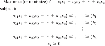
where
xi = decision variables
bi = constraint levels
cj = objective function coefficients
aij = constraint coefficients
Linear Programming Model Formulation
The Highlands Craft Store is a small craft operation that employs local artisans to produce clay bowls and mugs based on designs and colors from the 1700s and 1800s. The two primary resources used by the company are special pottery clay and skilled labor. Given these limited resources, the company wants to know how many bowls and mugs to produce each day to maximize profit.
The two products have the following resource requirements for production and selling price per item produced (i.e., the model parameters):
Product | Resource Requirements | ||
|---|---|---|---|
Labor (hr/unit) | Clay (lb/unit) | Revenue ($/unit) | |
Bowl | 1 | 4 | 40 |
Mug | 2 | 3 | 50 |
There are 40 hours of labor and 120 pounds of clay available each day. Formulate this problem as a linear programming model.
Solution
Management's decision is how many bowls and mugs to produce represented by the following decision variables.
x1 = number of bowls to produce
x2 = number of mugs to produce
The objective of the company is to maximize total revenue computed as the sum of the individual profits gained from each bowl and mug:
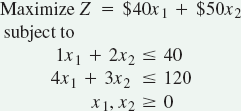
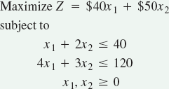
Maximize Z = $40x1 + 50x2
The model contains the constraints for labor and clay, which are
The less than or equal to inequality (≤) is used instead of an equality (=) because 40 hours of labor is a maximum that can be used, not an amount that must be used. However, constraints can be equalities (=), greater than or equal to inequalities (≥), or less than or equal to inequalities (≤).
The complete linear programming model for this problem can now be summarized as follows:
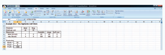
The solution of this model will result in numerical values for x1 and x2 that maximize total profit, Z, without violating the constraints. The solution that achieves this objective is x1 = 24 bowls and x2 = 8 mugs, with a corresponding revenue of $1360. We will discuss how we determined these values next.
A picture of how a solution is obtained for a linear programming model
The linear programming model in the previous section has characteristics common to all linear programming models. The mathematical relationships are additive; the model parameters are assumed to be known with certainty; the variable values are continuous (not restricted to integers); and the relationships are linear. Because of linearity, models with two decision variables (corresponding to two dimensions) can be solved graphically. Although graphical solution is cumbersome, it is useful in that it provides a picture of how a solution is derived.
• Graphical solution method: a method for solving a linear programming problem using a graph.
The basic steps in the graphical solution method are to plot the model constraints on a set of coordinates in a plane and identify the area on the graph that satisfies all the constraints simultaneously. The point on the boundary of this space that maximizes (or minimizes) the objective function is the solution. The following example illustrates these steps.
Graphical Solution
Determine the solution for Highlands Craft Store in Example S14.1:
The graph of the model constraints is shown in the following figure of the feasible solution space. The graph is produced in the positive quadrant since both decision variables must be positive or zero; that is, x1, x2 ≥ 0:
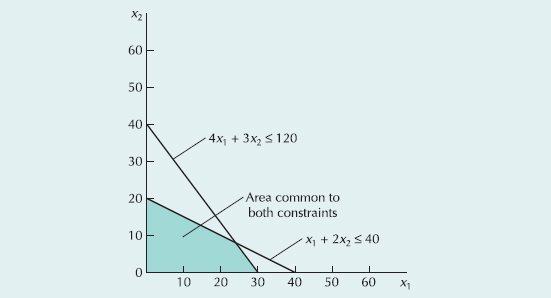
The first step is to plot the constraints on the graph. This is done by treating both constraints as equations (or straight lines) and plotting each line on the graph. A simple way to plot a line is to determine where it intersects the horizontal and vertical axes and draw a straight line connecting the points. The shaded area in the preceding figure is the area that is common to both model constraints. Therefore, this is the only area on the graph that contains points (i.e., values for x1 and x2) that will satisfy both constraints simultaneously. This area is the feasible solution space, because it is the only area that contains values for the variables that are feasible, or do not violate the constraints.
The second step in the graphical solution method is to locate the point in the feasible solution area that represents the greatest total revenue. We will plot the objective function line for an arbitrarily selected level of revenue. For example, if revenue, Z, is $800, the objective function is
• Feasible solution space: an area that satisfies all constraints in a linear programming model simultaneously.
$800 = 40x1 + 50x2
Plotting this line just as we plotted the constraint lines results in the graph showing the determination of the optimal point in the following figure. Every point on this line is in the feasible solution area and will result in a revenue of $800 (i.e., every combination of x1 and x2 on this line will give a Z value of $800). As the value of Z increases, the objective function line moves out through the feasible solution space away from the origin until it reaches the last feasible point on the boundary of the solution space and then leaves the solution space.
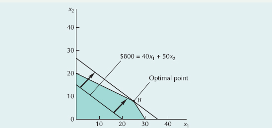
• Extreme points: corner points on the boundary of the feasible solution space.
• Optimal solution: the single best solution to a problem.
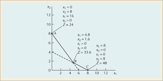
The solution point is always on this boundary, because the boundary contains the points farthest from the origin (i.e., the points corresponding to the greatest profit). Moreover, the solution point will not only be on the boundary of the feasible solution area, but it will be at one of the corners of the boundary where two constraint lines intersect. These corners (labeled A, B, and C in the following figure) are protrusions called extreme points. It has been proven mathematically that the optimal solution in a linear programming model will always occur at an extreme point. Therefore, in our example problem, the possible solution points are limited to the three extreme points A, B, and C. The optimal, or "one best," solution point is B, since the objective function touches it last before it leaves the feasible solution area.
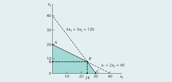
Because point B is formed by the intersection of two constraint lines, these two lines are equal at point B. Thus, the values of x1 and x2 at that intersection can be found by solving the two equations simultaneously:
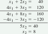
Thus,
The optimal solution at point B in the preceding figure is x1 = 24 bowls and x2 = 8 mugs. Substituting these values into the objective function gives the maximum revenue,
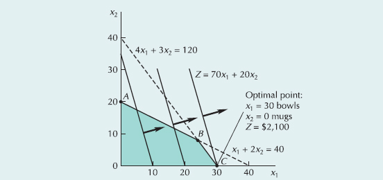
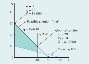
Given that the optimal solution will be at one of the extreme corner points A, B, or C, you can find the solution by testing each of the three points to see which results in the greatest revenue rather than by graphing the objective function and seeing which point it last touches as it moves out of the feasible solution area. The following figure shows the solution values for all three points A, B, and C and the amount of revenue, Z, at each point:
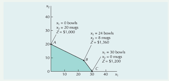
The objective function determines which extreme point is optimal, because the objective function designates the revenue that will accrue from each combination of x1 and x2 values at the extreme points. If the objective function had had different coefficients (i.e., different x1 and x2 profit values), one of the extreme points other than B might have been optimal.
Assume for a moment that the revenue for a bowl is $70 instead of $40 and the revenue for a mug is $20 instead of $50. These values result in a new objective function, Z = $70x1 + 20x2. If the model constraints for labor or clay are not changed, the feasible solution area remains the same, as shown in the following figure. However, the location of the objective function in this figure is different from that of the original objective function in the previous figure because the new profit coefficients give the linear objective function a new slope. Point C becomes optimal, with Z = $2100. This demonstrates one of the useful functions of linear programming—and model analysis in general—called sensitivity analysis: the testing of changes in the model parameters reflecting different operating environments to analyze the impact on the solution.
A Minimization Linear Programming Model
The Farmer's Hardware and Feed Store is preparing a fertilizer mix for a farmer who is preparing a field to plant a crop. The store will use two brands of fertilizer, Gro-Plus and Crop-Fast, to make the proper mix for the farmer. Each brand yields a specific amount of nitrogen and phosphate, as follows:
Brand | Chemical Contribution | |
|---|---|---|
Nitrogen (lb/bag) | Phosphate (lb/bag) | |
Gro-Plus | 2 | 4 |
Crop-Fast | 4 | 3 |
The farmer's field requires at least 16 pounds of nitrogen and 24 pounds of phosphate. Gro-Plus costs $6 per bag, and Crop-Fast costs $3. The store wants to know how many bags of each brand to purchase to minimize the total cost of fertilizing.
Formulate a linear programming model for this problem, and solve it using the graphical method.
Solution
This problem is formulated as follows:
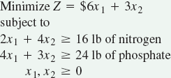
The graphical solution of the problem is shown in the following figure. Notice that the optimal solution, point A, occurs at the last extreme point the objective function touches as it moves toward the origin (point 0, 0).
• Simplex method: a mathematical procedure for solving a linear programming problem according to a set of steps.
Graphically determining the solution to a linear programming model can provide insight into how a solution is derived, but it is not generally effective or efficient. The traditional mathematical approach for solving a linear programming problem is a mathematical procedure called the simplex method. In the simplex method, the model is put into the form of a table, and then a number of mathematical steps are performed on the table. These mathematical steps are the same as moving from one extreme point on the solution boundary to another. However, unlike the graphical method, in which we simply searched through all the solution points to find the best one, the simplex method moves from one better solution to another until the best one is found.
The simplex method for solving linear programming problems is based, at least partially, on the solution of simultaneous equations and matrix algebra. In this supplement on linear programming, we are not going to provide a detailed presentation of the simplex method. It is a mathematically cumber-some approach that is very time-consuming even for very small problems of two or three variables and a few constraints. It includes a number of mathematical steps and requires numerous arithmetic computations, which frequently result in simple arithmetic errors when done by hand. Instead, we will demonstrate how linear programming problems are solved on the computer. Depending on the software used, the computer solution to a linear programming problem may be in the same form as a simplex solution. As such, we will review the procedures for setting up a linear programming model in the simplex format for solution.
Recall that the solution to a linear programming problem occurs at an extreme point where constraint equation lines intersect with each other or with the axis. Thus, the model constraints must all be in the form of equations (=) rather than inequalities (≥ or ≤).
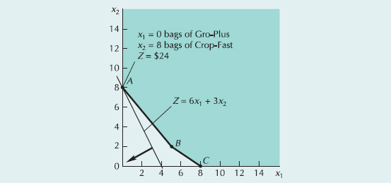
The procedure for transforming inequality constraints into equations is by adding a new variable, called a slack variable, to each constraint. For the Beaver Creek Pottery Company, the addition of a unique slack variable (si) to each of the constraint inequalities results in the following equations:
• Slack variable: a variable added to a linear programming constraint to make it an equality.
The slack variables, s1 and s2, will take on any value necessary to make the left-hand side of the equation equal to the right-hand side. If slack variables have a value in the solution, they generally represent unused resources. Since unused resources would contribute nothing to total revenue, they have a coefficient of zero in the objective function:
The graph in Figure S14.1 shows all the solution points in our Beaver Creek Pottery Company example with the values for decision and slack variables.
This example is a maximization problem with all ≤ constraints. A minimization problem with ≥ constraints requires a different adjustment. With a ≥ constraint, instead of adding a slack variable, we subtract a surplus variable. Whereas a slack variable is added and reflects unused resources, a surplus variable is subtracted and reflects the excess above a minimum resource-requirement level. Like the slack variable, a surplus variable is represented symbolically by si and must be nonnegative. For example, consider the following constraint from our fertilizer mix problem in Example S14.3:
• Surplus variable: a variable subtracted from a model constraint in a linear programming model in order to make it an equality.
Subtracting a surplus variable results in
2x1 + 4x2 – s1 = 16
The graph in Figure S14.2 shows all the solution points with the values for decision and surplus variables for the minimization problem in Example S14.3.
In this section we will demonstrate how to use Excel to solve the Highlands Craft Store model from Example S14.1.
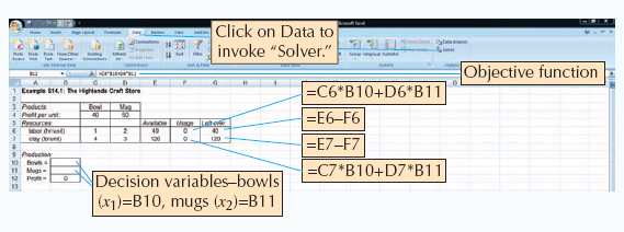
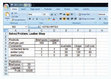
Exhibit S14.1 shows the Excel spreadsheet screen for Example S14.1 for the Highlands Craft Store. The values for bowls, mugs, and maximum profit are contained in cells B10, B11, and B12. They are currently empty since the problem has not yet been solved. The objective function for profit embedded in cell B12 is shown on the formula bar on the top of the screen. Similar formulas for the constraints for labor and clay are embedded in cells F6 and F7.
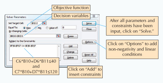
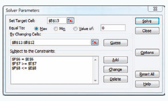
To solve this problem, first bring down the "Tools" window from the toolbar at the top of the screen and then select "Solver" from the list of menu items. (If Solver is not shown on the Tools menu, it can be activated by clicking on "Addins" on the Tools menu and then "Solver." If Solver is not available from the Add-ins menu, it must be installed on the Add-ins menu directly from the Office or Excel software.) The window for "Solver Parameters" will appear as shown in Exhibit S14.2. Initially all the windows on this screen are blank, and we must input the objective function cell, the cells representing the decision variables, and the cells that make up the model constraints.
When inputting the solver parameters as shown in Exhibit S14.2, we would first input the "target cell" that contains our objective function, which is B12 for our example. (Excel automatically inserts the "$" sign next to cell addresses; you should not type it in.) Next we indicate that we want to maximize the target cell by clicking on "Max." We achieve our objective "By Changing Cells" B10 and B11, which represent our model decision variables. The designation "B10:B11" means all the cells between B10 and B11 inclusive. We next input our model constraints by clicking on "Add," which will access a window for adding constraints.
After all the constraints have been added, there is one more necessary step before proceeding to solve the problem. Select "Options" from the "Solver Parameters" screen and then when the "Options" screen appears, click on "Assume Linear Models," then "OK." You can also click on "Assume Non-negative" to establish the non-negativity condition for the decision variables. This will allow you to eliminate the constraints, B10:B11 > = 0. Once the complete model is input, click on "Solve" in the upper right-hand corner of the "Solver Parameters" screen. First, a screen will appear entitled "Solver Results," which will provide you with the opportunity to select several different reports and then by clicking on "OK" the solution screen shown in Exhibit S14.3 will appear.
If there had been any slack left over for labor or clay, it would have appeared in column G on our spreadsheet under the heading "Left Over." In this case there are no slack resources left over.
We can also generate several reports that summarize the model results. When you click on "OK" from the "Solver" screen, an intermediate screen will appear before the original spreadsheet with the solution results. This screen is titled "Solver Results" and it provides an opportunity for you to select several reports, including an "Answer" report. This report provides a summary of the solution results.
The Excel solution also provides an additional useful piece of information called the "sensitivity report" as shown in Exhibit S14.4.
Notice the values 16 and 6 under the column labeled "Shadow Price" for the rows labeled "Labor usage" and "Clay usage." These values are the marginal values (also referred to as Shadow prices and dual values) of labor and clay in our problem. The marginal value is the amount the company would be willing to pay for one additional unit of a resource. For example, the marginal value of 16 for the labor constraint means that if one additional hour of labor could be obtained by the company, it would increase profit by $6. Likewise, if one additional pound of clay could be obtained, it would increase profit by $6. Sixteen dollars and $16 are the marginal values of labor and clay, respectively, for the company. The marginal value is not the original selling price of a resource; it is how much the company should pay to get more of the resource. The store should not be willing to pay more than $16 for an hour of labor because if it gets one more hour, profit will increase by only $16. The marginal value is helpful to the company in pricing resources and making decisions about securing additional resources.
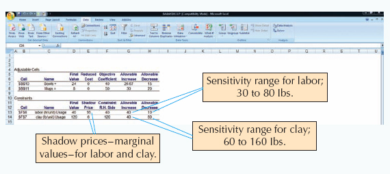
The marginal, or dual values do not hold for an unlimited supply of labor and clay. As the store increases (or reduces) the amount of labor or clay it has, the constraints change, which will eventually change the solution to a new point. Thus, the dual values are only good within a range of consistent values. These ranges are given under the column labeled "Allowable Increase" and "Allowable Decrease" in Exhibit S14.4. For example, the original amount of labor available is 40 hours. The dual value of $16 for one hour of labor holds if the available labor is between 30 and 80 hours. If there are more than 80 hours of labor, then a new solution point occurs and the dual value of $16 is no longer valid. The problem would have to be solved again to see what the new solution is and the new dual value.
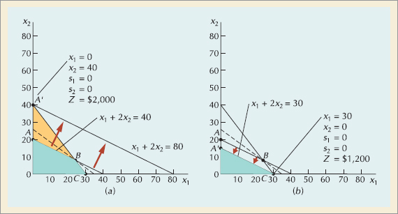
This can be observed graphically in Figure S14.3. If the labor hours are increased from 40 to 80 hours, the constraint line moves out and up. The new solution space is OA'C, and a new solution variable mix occurs at A', as shown in Figure S14.3a. At the original optimal point, B, both x1 and x2 are in the solution; however, at the new optimal point, A', only x2 is produced (i.e., x1 = 0, x2 = 40, s1 = 0, s2 = 0).
Thus, the upper limit of the sensitivity range for the labor constraint is 80 hours. At this value the solution mix changes such that bowls are no longer produced. Furthermore, as labor increases past 80 hours, s1 increases (i.e., slack hours are created). Similarly, if labor hours are decreased to 30 hours, the constraint line moves down and in. The new feasible solution space is OA'C, as shown in Figure S14.3b. The new optimal point is at C, where no mugs (x2) are produced. The new solution is x1 = 30, x2 = 0, s1 = 0, s2 = 0, and Z = $1200. Again, the variable mix is changed. Summarizing, the sensitivity range for the constraint quantity value for labor hours is between 30 and 80 hours as shown in the Excel spreadsheet in Exhibit S14.4.
A similar range of values exist for the clay constraint. The solution values are good for down to 60 lb and up to 160 lb as shown in Exhibit S14.4.
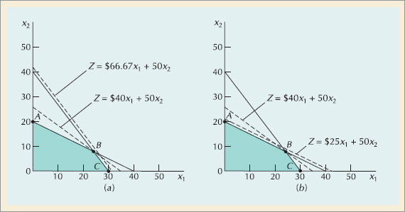
There are also sensitivity ranges for the objective function coefficients: "$40" for bowls and "$50" for mugs. The optimal solution point will remain the same if the profit for a bowl remains within $25 and $66.67, or if the profit for mugs remains between $30 and $80, as shown in the Excel spreadsheet in Exhibit S14.4. This can also be observed graphically in Figure S14.4.
If the profit for a bowl increases from $40 to $66.67, the objective function line rotates to a new location where it is parallel with the constraint line for clay as shown in Figure S14.4a. (At this new location, the objective function line and the constraint line for clay have the same slope). Both points B and C are now optimal. If the profit for bowls is increased greater than $66.67, then only point C will be optimal and we will have a new solution mix. Similarly, if the profit for a bowl is decreased to $25 as shown in Figure S14.4b, points A and B are both optimal. If the profit for a bowl is decreased to less than $25, only point A will be optimal and a new solution exists. Thus, the range for the profit for a bowl is between $25 and $66.67 as shown in the Excel spreadsheet in Exhibit S14.4. Over this range the current solution mix will remain optimal, and the marginal values are valid.
These sensitivity ranges for constraint values and objective function values provide managers with a convenient means for analyzing resource usage. The marginal value of resources lets managers know what their resources are worth as they make decisions, and the sensitivity ranges indicate the ranges over which the marginal values are valid. When using software like Excel, it is often just as easy to change different values in the linear programming model and see what happens. In either case, this points out a very useful feature of linear programming; it not only provides you with a possible solution or decision, but it also enables you to "experiment" with the model to test different operational scenarios.
Linear programming is one of several related quantitative techniques that are generally classified as mathematical programming models. Other quantitative techniques that fall into this general category include integer programming, nonlinear programming, and goal or multiobjective programming. These modeling techniques are capable of addressing a large variety of complex operational decisionmaking problems, and they are used extensively to do so by businesses and companies around the world. Computer software packages are available to solve most of these types of models, which greatly promotes their use.
constraints linear relationships of decision variables representing the restrictions placed on the decision situation by the operating environment.
decision variables mathematical symbols that represent levels of activity of an operation.
extreme points corner points, or protrusions, on the boundary of the feasible solution space in a linear programming model.
feasible solution space an area that satisfies all constraints in a linear programming model simultaneously.
graphical solution method a method for determining the solution of a linear programming problem using a two-dimensional graph of the model.
linear programming a technique for general decision situations in which the decision is to determine a level of operational activity in order to achieve an objective, subject to restrictions.
objective function a linear mathematical relationship that describes the objective of an operation in terms of decision variables.
optimal solution the single best solution to a problem.
simplex method a series of mathematical steps conducted within a tabular structure for solving a linear programming model.
slack variable a variable added to a linear programming ≤ constraint to make it an equality.
surplus variable a variable subtracted from a ≥ model constraint in a linear programming model in order to make it an equality.
A leather shop makes custom-designed, hand-tooled briefcases and luggage. The shop makes a $400 profit from each briefcase and a $200 profit from each piece of luggage. (The profit for briefcases is higher because briefcases require more hand-tooling.) The shop has a contract to provide a store with exactly 30 items per month. A tannery supplies the shop with at least 80 square yards of leather per month. The shop must purchase at least this amount but can order more. Each briefcase requires 2 square yards of leather; each piece of luggage requires 8 square yards of leather. From past performance, the shop owners know they cannot make more than 20 briefcases per month. They want to know the number of briefcases and pieces of luggage to produce in order to maximize profit. Formulate a linear programming model for this problem and solve it graphically.
SOLUTION
Step 1. Model formulation
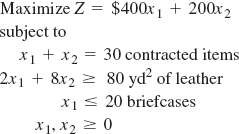
where
x1 = briefcases
x2 = pieces of luggage
Step 2. Graphical solution
Step 3. Model solution
The model solution obtained with Excel is shown as follows:
S14-1. Why is the term linear used in the name linear programming?
S14-2. Describe the steps one should follow in formulating a linear programming model.
S14-3. Summarize the steps for solving a linear programming model graphically.
S14-4. In the graphical analysis of a linear programming model, what occurs when the slope of the objective function is the same as the slope of one of the constraint equations?
S14-5. What are the benefits and limitations of the graphical method for solving linear programming problems?
S14-6. What constitutes the feasible solution area on the graph of a linear programming model?
S14-7. How is the optimal solution point identified on the graph of a linear programming model?
S14-8. Why does the coefficient of a slack variable equal zero in the objective function?
S14-1. Barrows Textile Mills produces two types of cotton cloth—denim and corduroy. Corduroy is a heavier grade of cotton cloth and, as such, requires 7.5 pounds of raw cotton per yard, whereas denim requires 5 pounds of raw cotton per yard. A yard of corduroy requires 3.2 hours of processing time; a yard of denim requires 3.0 hours. Although the demand for denim is practically unlimited, the maximum demand for corduroy is 510 yards per month. The manufacturer has 6500 pounds of cotton and 3000 hours of processing time available each month. The manufacturer makes a profit of $2.25 per yard of denim and $3.10 per yard of corduroy. The manufacturer wants to know how many yards of each type of cloth to produce to maximize profit.
Formulate and solve a linear programming model for this problem.
Solve this model using the graphical method.
S14-2. The Tycron Company produces three electrical products—clocks, radios, and toasters. These products have the following resource requirements:
Product | Resource Requirements | |
|---|---|---|
Cost/Unit | Labor Hours/Unit | |
Clock | $ 7 | 2 |
Radio | 10 | 3 |
Toaster | 5 | 2 |
The manufacturer has a daily production budget of $2000 and a maximum of 660 hours of labor. Maximum daily customer demand is for 200 clocks, 300 radios, and 150 toasters. Clocks sell for $15, radios, for $20, and toasters, for $12. The company desires to know the optimal product mix that will maximize profit.
Formulate and solve a linear programming model for this problem.
S14-3. The Seaboard Trucking Company has expanded its shipping capacity by purchasing 120 trucks and trailers from a competitor that went bankrupt. The company subsequently located 40 of the purchased trucks at each of its shipping warehouses in Charlotte, Memphis, and Louisville. The company makes shipments from each of these warehouses to terminals in St. Louis, Atlanta, and New York. Each truck is capable of making one shipment per week. The terminal managers have each indicated their capacity for extra shipments. The manager at St. Louis can accommodate 40 additional trucks per week, the manager at Atlanta can accommodate 60 additional trucks, and the manager at New York can accommodate 50 additional trucks. The company makes the following profit per truckload shipment from each warehouse to each terminal. The profits differ as a result of differences in products shipped, shipping costs, and transport rates.
Warehouse | Terminal | ||
|---|---|---|---|
St. Louis | Atlanta | New York | |
Charlotte | $1800 | $2100 | $1600 |
Memphis | 1000 | 700 | 900 |
Louisville | 1400 | 800 | 2200 |
The company wants to know how many trucks to assign to each route (i.e., warehouse to terminal) to maximize profit. Formulate a linear programming model for this problem and solve it.
S14-4. The Pinewood Cabinet and Furniture Company produces sofas, tables, and chairs at its plant in Greensboro, North Carolina. The plant uses three main resources to make furniture—wood, upholstery, and labor. The resource requirements for each piece of furniture and the total resources available weekly are as follows:
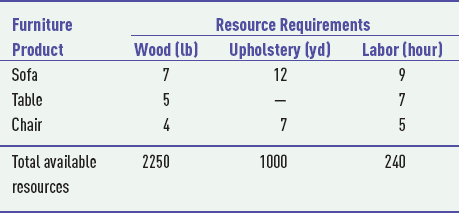
The furniture is produced on a weekly basis and stored in a warehouse until the end of the week, when it is shipped out. The warehouse has a total capacity of 500 pieces of furniture, however, a sofa takes up twice as much space as a table or chair. Each sofa earns $320 in profit, each table, $275, and each chair, $190. The company wants to know how many pieces of each type of furniture to make per week in order to maximize profit.
Formulate and solve a linear programming model for this problem.
S14-5. The Mystic Coffee Shop blends coffee on the premises for its customers. It sells three basic blends in one-pound bags: Special, Mountain Dark, and Mill Regular. It uses four different types of coffee to produce the blends: Brazilian, mocha, Colombian, and mild. The shop used the following blend recipe requirements:
Blend | Mix Requirements | Selling Price/lb |
|---|---|---|
Special | At least 40% Colombian, at least 30% mocha | $6.50 |
Dark | At least 60% Brazilian, no more than 10% mild | 5.25 |
Regular | No more than 60% mild, at least 30% Brazilian | 3.75 |
The cost of Brazilian coffee is $2.00 per pound, the cost of mocha is $2.75 per pound, the cost of Colombian is $2.90 per pound, and the cost of mild is $1.70 per pound. The shop has 110 pounds of Brazilian coffee, 70 pounds of mocha, 80 pounds of Colombian, and 150 pounds of mild coffee available per week. The shop wants to know the amount of each blend it should prepare each week in order to maximize profit.
Formulate and solve a linear programming model for this problem.
S14-6. A small metal-parts shop contains three machines—a drill press, a lathe, and a grinder—and has three operators, each certified to work on all three machines. However, each operator performs better on some machines than on others. The shop has contracted to do a big job that requires all three machines. The times required by the various operators to perform the required operations on each machine are summarized as follows:
Operator | Drill Press (min) | Lathe (min) | Grinder (min) |
|---|---|---|---|
1 | 22 | 18 | 35 |
2 | 29 | 30 | 28 |
3 | 25 | 36 | 18 |
The shop manager wants to assign one operator to each machine so that the total operating time for all three operators is minimized. Formulate and solve a linear programming model for this problem.
S14-7. The Tennessee Jack Distillery produces custom-blended whiskey. A particular blend consists of rye and bourbon whiskey. The company has received an order for a minimum of 400 gallons of the custom blend. The customer specified that the order must contain at least 40 percent rye and not more than 250 gallons of bourbon. The customer also specified that the blend should be mixed in the ratio of two parts rye to one part bourbon. The distillery can produce 500 gallons per week, regardless of the blend. The production manager wants to complete the order in one week. The blend is sold for $12 per gallon. The distillery company's cost per gallon is $4 for rye and $2 for bourbon. The company wants to determine the blend mix that will meet customer requirements and maximize profits.
Formulate and solve a linear programming model for this problem.
Solve the problem using the graphical method.
S14-8. A manufacturer of bathroom fixtures produces fiberglass bathtubs in an assembly operation consisting of three processes: molding, smoothing, and painting. The number of units that can be put through each process in an hour is as follows:
Process | Output (units/hr) |
|---|---|
Molding | 7 |
Smoothing | 12 |
Painting | 10 |
(Note: The three processes are continuous and sequential; thus, no more units can be smoothed or painted than have been molded.) The labor costs per hour are $8 for molding, $5 for smoothing, and $6.50 for painting. The company's labor budget is $3000 per week. A total of 120 hours of labor is available for all three processes per week. Each completed bathtub requires 90 pounds of fiberglass, and the company has a total of 10,000 pounds of fiberglass available each week. Each bathtub earns a profit of $175. The manager of the company wants to know how many hours per week to run each process in order to maximize profit. Formulate and solve a linear programming model for this problem.
S14-9. A refinery blends four petroleum components into three grades of gasoline—regular, premium, and super. The maximum quantities available of each component and the cost per barrel are as follows:
Component | Maximum Barrels Available/day | Cost (barrel) |
|---|---|---|
1 | 5000 | $9.00 |
2 | 2400 | 7.00 |
3 | 4000 | 12.00 |
4 | 1500 | 6.00 |
To ensure that each gasoline grade retains certain essential characteristics, the refinery has put limits on the percentage of the components in each blend. The limits as well as the selling prices for the various grades are as follows:
Grade | Component Specifications | Selling Price (barrel) |
|---|---|---|
Super | Not less than 40% of 1 Not more than 20% of 2 Not less than 30% of 3 | $12.00 |
Premium | Not less than 40% of 3 Not more than 50% of 2 | 18.00 10.00 |
Regular | Not less than 10% of 1 |
The refinery wants to produce at least 3000 barrels each of super and premium and 4000 barrels of regular. Management wishes to determine the optimal mix of the four components that will maximize profit. Formulate and solve a linear programming model for this problem.
S14-10. The Home Improvement Building Supply Company has received the following order for boards in three lengths:
Length | Order (quantity) |
|---|---|
7 feet | 700 boards |
9 feet | 1200 boards |
10 feet | 500 boards |
The company has 25-foot standard-length boards in stock. Therefore, the standard-length boards must be cut into the lengths necessary to meet order requirements. Naturally, the company wishes to minimize the number of standard-length boards used. The company must, therefore, determine how to cut up the 25-foot boards in order to meet the order requirements and minimize the number of standard-length boards used.
Formulate and solve a linear programming model for this problem.
When a board is cut in a specific pattern, the amount of board left over is referred to as trim loss. Reformulate and solve the linear programming model for this problem, assuming that the objective is to minimize trim loss rather than to minimize the total number of boards used.
S14-11. IT Computer Services assembles its own brand of personal computers from component parts it purchases over-seas and domestically. IT sells most of its computers locally to different departments at State University as well as to individuals and businesses in the immediate geographic region.
IT has enough regular production capacity to produce 160 computers per week. It can produce an additional 50 computers with overtime. The cost of assembly, inspecting, and packaging a computer during regular time is $190. Overtime production of a computer costs $260. Further, it costs $5 per computer per week to hold a computer in inventory for future delivery. IT wants to be able to meet all customer orders with no shortages in order to provide quality service. IT's order schedule for the next 6 weeks is as follows:
Week | Computer orders |
|---|---|
1 | 105 |
2 | 170 |
3 | 230 |
4 | 180 |
5 | 150 |
6 | 250 |
IT Computers wants to determine a schedule that will indicate how much regular and overtime production it will need each week in order to meet its orders at the minimum cost. The company wants no inventory left over at the end of the six-week period. Formulate and solve a linear programming model for this problem.
S14-12. The manager of Biggs Department Store has four employees available to assign to three departments in the store: lamps, sporting goods, and linen. The manager wants each of these departments to have at least one employee but not more than two. Therefore, two departments will be assigned one employee, and one department will be assigned two. Each employee has different areas of expertise, which are reflected in the following average daily sales record for each employee from previous experience in each department:
Employee | Department | ||
|---|---|---|---|
Lamps | Sporting Goods | Linen | |
1 | $130 | $190 | $ 90 |
2 | 275 | 300 | 100 |
3 | 180 | 225 | 140 |
4 | 200 | 120 | 160 |
The manager wishes to know which employee(s) to assign to each department in order to maximize expected sales. Formulate and solve a linear programming model for this problem.
S14-13. Dr. Beth McKenzie, the head administrator at Washington County Regional Hospital, must determine a schedule for nurses to make sure there are enough nurses on duty throughout the day. During the day, the demand for nurses varies. Beth has broken the day into twelve 2-hour periods. The slowest time of the day encompasses the three periods from 12:00 a.m. to 6:00 a.m., which, beginning at midnight, require a minimum of 30, 20, and 40 nurses, respectively. The demand for nurses steadily increases during the next four daytime periods. Beginning with the 6:00 a.m.–8:00 a.m. period, a minimum of 50, 60, 80, and 90 nurses are required for these four periods, respectively. After 2:00 p.m., the demand for nurses decreases during the afternoon and evening hours. For the five 2-hour periods beginning at 2:00 p.m., and ending at midnight, 70, 70, 60, 50, and 40 nurses are required, respectively. A nurse reports for duty at the beginning of one of the 2-hour periods and works 8 consecutive hours (which is required in the nurses' contract). Dr. McKenzie wants to determine a nursing schedule that will meet the hospital's minimum requirements throughout the day while using the minimum number of nurses. Formulate and solve a linear programming model for this problem.
S14-14. Grass Unlimited is a lawn care and maintenance company. One of its services is to seed new lawns as well as bare areas or damaged areas in established lawns. The company uses three basic grass seed mixes it calls Home 1, Home 2, and Commercial 3. It uses three kinds of grass seed—tall fescue, mustang fescue, and bluegrass. The requirements for each grass mix are as follows:
Mix | Mix Requirements |
|---|---|
Home 1 | No more than 50% tall fescue At least 20% mustang fescue |
Home 2 | At least 30% bluegrass At least 30% mustang fescue No more than 20% tall fescue |
Commercial 3 | At least 50% but no more than 70% tall fescue At least 10% bluegrass |
The company believes it needs to have at least 1500 pounds of Home 1 mix, 900 pounds of Home 2 mix, and 2400 pounds of Commercial 3 seed mix on hand. A pound of tall fescue costs the company $1.70, a pound of mustang fescue costs $2.80, and a pound of bluegrass costs $3.25. The company wants to know how many pounds of each type of grass seed to purchase in order to minimize cost. Formulate a linear programming model for this problem.
S14-15. A jewelry store makes necklaces and bracelets from gold and platinum. The store has developed the following linear programming model for determining the number of necklaces and bracelets (x1 and x2) to make in order to maximize profit:
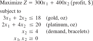
Solve this model graphically.
The maximum demand for bracelets is 4. If the store produces the optimal number of bracelets and necklaces, will the maximum demand for bracelets be met? If not, by how much will it be missed?
What profit for a necklace would result in no bracelets being produced, and what would be the optimal solution for this problem?
S14-16. The Copperfield Mining Company owns two mines, which produce three grades of ore: high, medium, and low. The company has a contract to supply a smelting company with 12 tons of high-grade ore, 8 tons of medium-grade ore, and 24 tons of low-grade ore. Each mine produces a certain amount of each type of ore each hour it is in operation. The company has developed the following linear programming model to determine the number of hours to operate each mine (x1 and x2) so that contracted obligations can be met at the lowest cost:
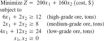
Solve this model graphically.
Solve the model using Excel.
S14-17. A manufacturing firm produces two products. Each product must go through an assembly process and a finishing process. The product is then transferred to the warehouse, which has space for only a limited number of items. The following linear programming model has been developed for determining the quantity of each product to produce in order to maximize profit:
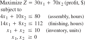
Solve this model graphically.
Assume that the objective function has been changed to Z = 90x1 + 70x2. Determine the slope of each objective function and discuss what effect these slopes have on the optimal solution.
S14-18. The Admissions Office at Tech wants to determine how many instate and out-of-state students to accept for next fall's entering freshman class. Tuition for an in-state student is $7600 per year while out-of-state tuition is $22,500 per year. A total of 12,800 in-state and 8100 out-of-state freshman have applied for next fall, and Tech does not want to accept more than 3500 students. However, since Tech is a state institution, the state mandates that it can accept no more than 40% out-of-state students. From past experience the admissions office knows that 12% of in-state students and 24% of out-of-state students will drop out during their first year. Tech wants to maximize total tuition while limiting the total attrition to 600 first-year students.
Formulate a linear programming model for this problem.
Solve this model using graphical analysis.
Solve this problem using Excel.
S14-19. Janet Lopez is establishing an investment portfolio that will include stock and bond funds. She has $720,000 to invest, and she does not want the portfolio to include more than 65% stocks. The average annual return for the stock fund she plans to invest in is 18%, while the average annual return for the bond fund is 6%. She further estimates that the most she could lose in the next year in the stock fund is 22%, while the most she could lose in the bond fund is 5%. To reduce her risk she wants to limit her potential maximum losses to $100,000.
Formulate a linear programming model for this problem.
Solve this model using graphical analysis.
Solve this problem using Excel.
S14-20. Professor Wang teaches two sections of operations management, which combined will result in 130 final exams to be graded. Professor Wang has two graduate assistants (GAs), James and Ann, who will grade the final exam. There is a 3-day period between the time the exam is administered and when final grades must be posted. During this period James has 14 hours available and Ann has 12 available hours to grade the exams. It takes James an average of 8.4 minutes to grade an exam, and it takes Sarah 15 minutes to grade an exam; however, James's exams will have errors that will require Professor Wang to ultimately regrade 12% of his exams, while only 5% of Ann's exams will require regrading. Professor Wang wants to know how many exams to assign to each GA to grade in order to get all of them graded, but she also wants to minimize the number of exams that she will be required to regrade.
Formulate a linear programming model for this problem.
Solve this model using graphical analysis.
Solve this model using Excel.
If Professor Wang could hire James or Ann to work one more hour, which should she choose? What would be the effect of hiring the selected GA for one additional hour?
S14-21. The Star City Café at the campus student center serves two coffee blends it brews daily, Morning Blend and Study Break. Each is a blend of three high-quality coffees from Brazil, Tanzania, and Guatemala. The Cafe has 5 lbs. of each of these coffees available each day. Each pound of coffee will produce sixteen 16-oz cups of coffee, and the Cafe has enough brewing capacity to brew 25 gl. of the two coffee blends each day. Morning Blend includes 25% Brazilian, 30% Tanzanian, and 45% Guatemalan, while Study Break is a blend of 55% Brazilian, 15% Tanzanian, and 30% Guatemalan. The shop sells one and a half times more Morning Blend than Study Break each day. Morning Blend sells for $1.95 per cup, and Coastal sells for $1.70 per cup. The manager wants to know the number of cups of each blend to sell each day in order to maximize sales.
Formulate a linear programming model for this problem.
Solve this model using graphical analysis.
Solve this model using Excel.
If the Café could get one more pound of coffee, which one should it be? What would be the effect on sales of getting one more pound of this coffee?
Would it benefit the shop to increases its brewing capacity from 25 gallons to 30 gallons?
Should the Cafe spend $25 per day on advertising if it would increase the relative demand for Morning Blend to twice that of Study Break?
S14-22. Breathtakers, a health and fitness center, operates a morning fitness program for senior citizens. The program includes aerobic exercise, either swimming or step exercise, followed by a healthy breakfast in its dining room. The dietitian of Breathtakers wants to develop a breakfast that will be high in calories, calcium, protein, and fiber, which are especially important to senior citizens, but low in fat and cholesterol. She also wants to minimize cost. She has selected the following possible food items, with individual nutrient contributions and cost from which to develop a standard breakfast menu.
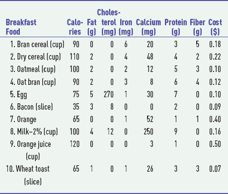
The dietitian wants the breakfast to include at least 420 calories, 5 milligrams of iron, 400 milligrams of calcium, 20 grams of protein, and 12 grams of fiber. Furthermore, she wants to limit fat to no more than 20 grams and cholesterol to 30 milligrams. Formulate the linear programming model for this problem and solve.
S14-23. The Midland Tool Shop has four heavy presses it uses to stamp out prefabricated metal covers and housings for electronic consumer products. All four presses operate differently and are of different sizes. Currently, the firm has a contract to produce three products. The contract calls for 450 units of product 1; 600 units of product 2; and 320 units of product 3. The time (minutes) required for each product to be produced on each machine is as follows:
Product | Machine | |||
|---|---|---|---|---|
1 | 2 | 3 | 4 | |
1 | 35 | 41 | 34 | 39 |
2 | 40 | 36 | 32 | 43 |
3 | 38 | 37 | 33 | 40 |
Machine 1 is available for 150 hours, machine 2 for 240 hours, machine 3 for 200 hours, and machine 4 for 250 hours. The products also result in different profits according to the machine they are produced on because of time, waste, and operating cost. The profit per unit per machine for each product is summarized as follows:
Product | Machine | |||
|---|---|---|---|---|
1 | 2 | 3 | 4 | |
1 | $7.8 | 7.8 | 8.2 | 7.9 |
2 | 6.7 | 8.9 | 9.2 | 6.3 |
3 | 8.4 | 8.1 | 9.0 | 5.8 |
The company wants to know how many units of each product to produce on each machine in order to maximize profit.
Formulate and solve a linear programming model for this problem.
S14-24. The Willow Run Coal Company operates three mines in Kentucky and West Virginia and supplies coal to four utility power plants along the East Coast. The cost of shipping coal from each mine to each plant, the capacity at each of the four mines, and demand at each plant are shown in the following table:
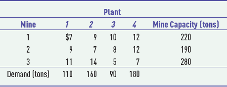
The cost of mining and processing coal is $62 per ton at mine 1, $67 per ton at mine 2, and $75 per ton at mine 3. The percentage of ash and sulfur content per ton of coal at each mine is as follows:
Mine | % Ash | % Sulfur |
|---|---|---|
1 | 9 | 6 |
2 | 5 | 4 |
3 | 4 | 3 |
Each plant has different cleaning equipment. Plant 1 requires that the coal it receives can have no more than 6% ash and 5% sulfur; plant 2 coal can have no more than 5% ash and sulfur combined; plant 3 can have no more than 5% ash and 7% sulfur; and plant 4 can have no more than 6% ash and sulfur combined. The company wants to determine the amount of coal to produce at each mine and ship to its customers that will minimize its total cost.
Formulate and solve a linear programming model for this problem.
S14-25. Armco, Inc., is a manufacturing company that has a contract to supply a customer with parts from April through September. However, Armco does not have enough storage space to store the parts during this period, so it needs to lease extra warehouse space during the 6-month period. Following are Armco's space requirements:
Month | Required Space (ft2) |
|---|---|
April | 47,000 |
May | 35,000 |
June | 52,000 |
July | 27,000 |
August | 19,000 |
September | 15,000 |
The rental agent Armco is dealing with has provided it with the following cost schedule for warehouse space. This schedule shows that the longer the space is rented the cheaper it is. For example, if Armco rents space for all six months, it costs $1.00/ft2 per month, whereas if it rents the same space for only one month, it costs $1.70/ft2 per month.
Rental Period (months) | $/ft2/mo |
|---|---|
6 | 1.00 |
5 | 1.05 |
4 | 1.10 |
3 | 1.20 |
2 | 1.40 |
1 | 1.70 |
Armco can rent any amount of warehouse space on a monthly basis at any time for any number of (whole) months. Armco wants to determine the least costly rental agreement that will exactly meet its space needs each month and avoid any unused space.
Formulate and solve a linear programming model for this problem.
Suppose that Armco decided to relax its restriction that is rent exactly the space it needs every month such that it would rent excess space if it were cheaper. How would this affect the optimal solution?
S14-26. Fun 'n Games is a large discount toy store in Fashion City Mall. The store typically has slow sales in the summer months that increase dramatically and rise to a peak at Christmas. However, during the summer and fall, the store must build up its inventory to have enough stock for the Christmas season. In order to purchase and build up its stock during the months when its revenues are low, the store borrows money.
Following is the store's projected revenue and liabilities schedule for July through December (where revenues are received and bills are paid at the first of each month).
Month | Revenues | Liabilities |
|---|---|---|
July | $20,000 | $60,000 |
August | 30,000 | 60,000 |
September | 40,000 | 80,000 |
October | 50,000 | 30,000 |
November | 80,000 | 30,000 |
December | 100,000 | 20,000 |
At the beginning of July the store can take out a six-month loan that carries an 11% interest rate and must be paid back at the end of December. (The store cannot reduce its interest payment by paying back the loan early.) The store can also borrow money monthly at a rate of 5% interest per month. Money borrowed on a monthly basis must be paid back at the beginning of the next month. The store wants to borrow enough money to meet its cash flow needs while minimizing its cost of borrowing.
Formulate and solve a linear programming model for this problem.
What would be the effect on the optimal solution if the store could secure a 9% interest rate for a 6-month loan from another bank?
S14-27. The Bassone Boat Company manufactures the Water Wiz bass fishing boat. The company purchases the engines it installs in its boats from the Margine Company that specializes in marine engines. Bassone has the following production scheduling for April, May, June, and July:
Month | Production |
|---|---|
April | 60 |
May | 85 |
June | 100 |
July | 120 |
Mar-gine usually manufactures and ships engines to Bassone during the month the engines are due. However, from April through July Margine has a large order with another boat customer and it can only manufacture 40 engines in April, 60 in May, 90 in June, and 50 in July. Margine has several alternative ways to meet Bassone's production schedule. It can produce up to 30 engines in January, February, and March and carry them in inventory at a cost of $50 per engine per month until it ships them to Bassone. For example, Mar-gine could build an engine in January and ship it to Bassone in April incurring $150 in inventory charges. Mar-gine can also manufacture up to 20 engines in the month they are due on an overtime basis with an additional cost of $400 per engine. Mar-gine wants to determine the least costly production schedule that will meet Bassone's schedule.
Formulate and solve a linear programming model for this problem.
If Mar-gine is able to increase its production capacity in January, February, and March from 30 to 40 engines, what would be the effect on the optimal solution?
S14-28. Far North Outfitters is a retail phone-catalogue company that specializes in outdoor clothing and equipment. A phone station at the company will be staffed with either full-time operators or temporary operators 8 hours per day. Full-time operators, because of their experience and training, process more orders and make fewer mistakes than temporary operators. However, temporary operators are cheaper because of a lower wage rate, and they are not paid benefits. A full-time operator can process about 360 orders per week, whereas a temporary operator can process about 270 orders per week. A full-time operator will average 1.1 defective orders per week, and a part-time operator will incur about 2.7 defective orders per week. The company wants to limit defective orders to 200 per week. The cost of staffing a station with full-time operators is $610 per week, and the cost of a station with part-time operators is $450 per week. Using historical data and forecasting techniques, the company has developed estimates of phone orders for an eight-week period as follows:
Weeks | Orders |
|---|---|
1 | 19,500 |
2 | 21,000 |
3 | 25,600 |
4 | 27,200 |
5 | 33,400 |
6 | 29,800 |
7 | 27,000 |
8 | 31,000 |
The company does not want to hire or dismiss full-time employees after the first week (i.e., the company wants a constant group of full-time operators over the eight-week period). The company wants to determine how many full-time operators it needs and how many temporary operators to hire each week in order to meet weekly demand while minimizing labor costs.
Formulate and solve a linear programming model for this problem.
Far North Outfitters is going to alter its staffing policy. Instead of hiring a constant group of full-time operators for the entire eight-week planning period, it has decided to hire and add full-time operators as the eight-week period progresses, although once it hires full-time operators it will not dismiss them. Reformulate the linear programming model to reflect this altered policy and solve to determine the cost savings (if any).
S14-29. Eyewitness News is shown on channel 5 Monday through Friday evenings from 5:00 P.M to 6:00 P.M. During the hour-long broadcast, 18 minutes are allocated to commercials. The remaining 42 minutes of airtime are allocated to single or multiple time segments for local news and features, national news, sports, and weather. The station has learned through several viewer surveys that viewers do not consistently watch the entire news program; they focus on some segments more closely than others. For example, they tend to pay more attention to the local weather than the national news (because they know they will watch the network news following the local broadcast). As such, the advertising revenues generated for commercials shown during the different broadcast segments are $850/minute for local news and feature story segments, $600/minute for national news, $750/minute for sports, and $1000/minute for the weather. The production cost for local news is $400/minute, the cost for national news is $100/minute, for sports the cost is $175/minute and for weather it is $90/minute. The station budgets $9000 per show for production costs. The station's policy is that the broadcast time devoted to local news and features must be at least 10 minutes but no more than 25 minutes while national news, sports, and weather must each have segments of at least 5 minutes but no more than 10 minutes. Commercial time must be limited to no more than 6 minutes for each of the four broadcast segment types. The station manager wants to know how many minutes of commercial time and broadcast time to allocate to local news, national news, sports and weather in order to maximize advertising revenues.
Formulate and solve a linear programming model for this problem.
S14-30. The McCoy Family raises cattle on their farm in Virginia. They also have a large garden in which they grow ingredients for making two types of relish—chow-chow and tomato. These they sell in 16-ounce jars at local stores and craft fairs in the fall. The profit for a jar of chow-chow is $2.25, and the profit for a jar of tomato relish is $1.95. The main ingredients in each relish are cabbage, tomatoes, and onions. A jar of chow-chow must contain at least 60% cabbage, 5% onions, and 10% tomatoes, and a jar of tomato relish must contain at least 50% tomatoes, 5% onions, and 10% cabbage. Both relishes contain no more than 10% onions. The family has enough time to make no more than 700 jars of relish. In checking sales records for the past five years, they know that they will sell at least 30% more chow-chow than tomato relish. They will have 300 pounds of cabbage, 350 pounds of tomatoes, and 30 pounds of onions available. The McCoy family wants to know how many jars of relish to produce to maximize profits.
Formulate and solve a linear programming model for this problem.
S14-31. The Big Max grocery store sells three brands of milk in half-gallon cartons—its own brand, a local dairy brand, and a national brand. The profit from its own brand is $0.97 a carton, the profit from the local dairy brand is $0.83 per carton, and the profit from the national brand is $0.69 per carton. The total refrigerated shelf space allotted to half-gallon cartons of milk is 36 square feet per week. A half-gallon carton takes up 16 square inches of shelf space. The store manager knows that they always sell more of the national brand than the local dairy brand and their own brand combined each week, and they always sell at least three times as much of the national brand as their own brand each week. In addition, the local dairy can supply only 10 dozen cartons per week. The store manager wants to know how many half-gallon cartons of each brand to stock each week in order to maximize profit.
Formulate and solve a linear programming model for this problem.
If Big Max could increase its shelf space for halfgallon cartons of milk, how much would profit increase per carton?
If Big Max could get the local dairy to increase the amount of milk it could supply each week, would it increase profit?
Big Max is considering discounting its own brand in order to increase sales. If it does so, it would decrease the profit margin for its own brand to $0.86 per carton but it would cut the demand for the national brand relative to its own brand in half. Discuss whether or not the store should implement the price discount.
S14-32. John Davis owns Eastcoasters, a bicycle shop in Millersville. Most of John's bicycle sales are customer orders; however, he also stocks bicycles for walk-in customers. He stocks three types of bicycles—road racing, cross country, and mountain. The cost of a road racing bike is $1200, a cross-country bike costs $1700, and a mountain bike costs $900. He sells road racing bikes for $1800, cross-country bikes for $2100, and mountain bikes for $1200. He has $12,000 available this month to purchase bikes. Each bike must be assembled; a road racing bike requires 8 hours to assemble, a cross-country bike requires 12 hours, and a mountain bike requires 16 hours. He estimates that he and his employees have 120 hours available to assemble bikes. He has enough space in his store to order 20 bikes this month. Based on past sales, John wants to stock at least twice as many mountain bikes as the other two combined because they sell better.
Formulate and solve a linear programming model for this problem.
Should John try to increase his budget for purchasing bikes, get more space to stock bikes, or get additional labor hours to assemble bikes? Why?
If, in (a), John hired an additional worker for 30 hours at $10/hr, how much additional profit would he make, if any?
If John purchased a cheaper cross-country bike for $1200 and sold it for $1900 would it affect the original solution?
S14-33. The Townside Food Services Company delivers fresh sandwiches each morning to vending machines throughout the city. Workers assemble sandwiches from previously prepared ingredients through the night for morning delivery. The company makes three kinds of sandwiches: ham and cheese, bologna, and chicken salad. A ham and cheese sandwich requires a worker 0.45 minute to assemble, a bologna sandwich requires 0.41 minute, and a chicken salad sandwich 0.50 minute to make. The company has 960 available minutes each night for sandwich assembly. The company has available vending machine capacity for 2000 sandwiches each day. The profit for a ham and cheese sandwich is $0.35, the profit for a bologna sandwich is $0.42, and the profit for a chicken salad sandwich is $0.37. The company knows from past sales records that their customers buy as many or more of the ham and cheese sandwiches than the other two sandwiches combined, but they need to have a variety of sandwiches available, so they stock at least 200 of each. Townside management wants to know how many of each sandwich it should stock in order to maximize profit.
Formulate and solve a linear programming model for this problem.
If Townside Food Service could hire another worker and increase its available assembly time by 480 minutes, or increase its vending machine capacity by 100 sandwiches, which should it do? Why? How much additional profit would your decision result in?
What would be the effect on the optimal solution if the requirement that at least 200 sandwiches of each kind be stocked was eliminated? Compare the profit between the optimal solution and this solution, and indicate which solution you would recommend.
What would be the effect on the optimal solution if the profit for a ham and cheese sandwich was increased to $0.40? $0.45?
S14-34. The admissions office at State University wants to develop a planning model for next year's entering freshman class. The university has 4500 available openings for freshman. Tuition is $8600 for an in-state student and $19,200 for an out-of-state student. The university wants to maximize the money it receives from tuition, but by state mandate it can admit no more than 47% out-of-state students. Also, each college in the university must have at least 30% in-state students in its freshman class. In order to be ranked in several national magazines, it wants the freshman class to have an average SAT score of 1150. Following are the average SAT scores for last year's freshman class for in-state and out-of-state students in each college in the university, plus the maximum size of the freshman class for each college.
College | In-State | Average SAT Scares Out-of-State | Total Capacity |
|---|---|---|---|
1. Architecture | 1350 | 1460 | 470 |
2. Arts & Sciences | 1010 | 1050 | 1300 |
3. Agriculture | 1020 | 1110 | 240 |
4. Business | 1090 | 1180 | 820 |
5. Engineering | 1360 | 1420 | 1060 |
6. Human Resources | 1000 | 1400 | 610 |
Formulate and solve a linear programming model that will determine the number of in-state and out-of-state students that should enter each college.
If the solution in part (a) does not achieve the maximum freshman class size, discuss how you might adjust the model to reach this class size.
S14-35. Vantage Systems is a consulting firm that develops e-commerce systems and Web sites for its clients. It has six available consultants and eight client projects under contract. The consultants have different technical abilities and experience, and as a result the company charges different hourly rates for their services. Also, the consultants' skills are more suited for some projects than for others, and clients sometimes prefer some consultants over others. The suitability of a consultant for a project is rated according to a five-point scale, where 1 is the worst and 5 is the best. The following table shows the rating for each consultant for each project as well as the hours available for each consultant, and the contracted hours and maximum budget for each project.
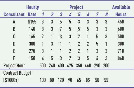
The company wants to know how many hours to assign each consultant to each project that will best utilize the consultants' skills while meeting the clients' needs.
Formulate and solve a linear programming model for this problem.
If the company's objective is to maximize revenue while ignoring client preferences and consultant compatibility, will this change the solution in (b)?
S14-36. East Coast Airlines operates a hub at the Pittsburgh International Airport. During the summer, the airline schedules seven flights daily from Pittsburgh to Orlando and ten flights daily from Orlando to Pittsburgh according to the following schedule.
Flight | Leave Pittsburgh | Arrive Orlando | Flight | Leave Orlando | Arrive Pittsburgh |
|---|---|---|---|---|---|
1 | 6 a.m. | 9 a.m. | A | 6 a.m. | 9 a.m. |
2 | 8 a.m. | 11 a.m. | B | 7 a.m. | 10 a.m. |
3 | 9 a.m. | Noon | C | 8 a.m. | 11 a.m. |
4 | 3 p.m. | 6 p.m. | D | 10 a.m. | 1 p.m. |
5 | 5 p.m. | 8 p.m. | E | Noon | 3 p.m. |
6 | 7 p.m. | 10 p.m. | F | 2 p.m. | 5 p.m. |
7 | 8 p.m. | 11 p.m. | G | 3 p.m. | 6 p.m. |
H | 6 p.m. | 9 p.m. | |||
I | 7 p.m. | 10 p.m. | |||
J | 9 p.m. | Midnight |
The flight crews live in Pittsburgh or Orlando, and each day a new crew must fly one flight from Pittsburgh to Orlando and one flight from Orlando to Pittsburgh. A crew must return to its home city at the end of each day. For example, if a crew originates in Orlando and flies a flight to Pittsburgh, it must then be scheduled for a return flight from Pittsburgh back to Orlando. A crew must have at least one hour between flights at the city where it arrives. Some scheduling combinations are not possible; for example, a crew on flight 1 from Pittsburgh cannot return on flights A, B, or C from Orlando. It is also possible for a flight to ferry one additional crew to a city in order to fly a return flight, if there are not enough crews in that city.
The airline wants to schedule its crews in order to minimize the total amount of crew ground time (i.e., the time the crew is on the ground between flights). Excessive ground time for a crew lengthens its work day, is bad for crew morale, and is expensive for the airline. Formulate a linear programming model to determine a flight schedule for the airline and solve using Excel. How many crews need to be based in each city? How much ground time will each crew experience?
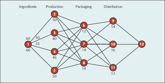
S14-37. The National Cereal Company produces a Light-Snak cereal package with a selection of small pouches of four different cereals—Crunchies, Toasties, Snakmix, and Granolies. Each cereal is produced at a single production facility and then shipped to three packaging facilities where the four different cereal pouches are combined into a single box. The boxes are then sent to one of three distribution centers where they are combined to fill customer orders and shipped. The diagram at the top of the next page shows the weekly flow of the product through the production, packaging, and distribution facilities (referred to as a supply chain).
Ingredients capacities (per 1000 pouches) per week are shown along branches 1–2, 1–3, 1–4, and 1–5. For example, ingredients for 60,000 pouches are available at the production facility as shown on branch 1–2. The weekly production capacity at each plant (in 1000s of pouches) is shown at nodes 2, 3, 4, and 5. The packaging facilities at nodes 6, 7, and 8 and the distribution centers at nodes 9, 10, and 11 have capacities for boxes (1000s) as shown.
The various production, packaging and distribution costs per unit at each facility are shown in the following table.
Facility | 2 | 3 | 4 | 5 | 6 | 7 | 8 | 9 | 10 | 11 |
|---|---|---|---|---|---|---|---|---|---|---|
Unit cost | $0.17 | 0.20 | 0.18 | 0.16 | 0.26 | 0.29 | 0.27 | 0.12 | 0.11 | 0.14 |
Weekly demand for the Light-Snak product is 37,000 boxes.
Formulate and solve a linear programming model that indicates how much product is produced at each facility that will meet weekly demand at the minimum cost.
S14-38. Grove Food Products Company has contracted with apple growers in Wisconsin, lowa, and Virginia to purchase apples, which the company then ships to its plants in Ohio and Alabama where it is processed into apple juice. Each bushel of apples will produce two gallons of apple juice. The juice is canned and bottled at the plants and shipped by rail and truck to warehouse/distribution centers in Pennsylvania, Tennessee, and North Carolina. The shipping costs per bushel from the farms to the plants and the shipping costs per gallon from the plants to the distribution centers are summarized in the following tables.
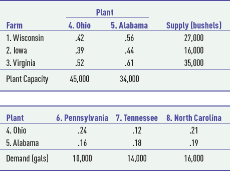
Formulate and solve a linear programming model to determine the optimal shipments from the farms to the plants and from the plants to the distribution centers that will minimize total shipping costs.
S14-39. Valley Electric Company generates electrical power at four coal-fired power plant in Pennsylvania, West Virginia, Kentucky and Virginia. The company purchases coal from six producers in southwestern Virginia, West Virginia and Kentucky. Valley Electric has fixed contracts for coal delivery from the following three coal producers:
Coal Producer | Tons | Cost ($/ton) | Million BTUs/ton |
|---|---|---|---|
APCO | 180,000 | 24 | 27.2 |
Balfour | 315,000 | 27 | 28.1 |
Cannon | 340,800 | 26 | 26.6 |
The power-producing capabilities of the coal produced by these suppliers differs according to the quality of the coal. For example, coal produced by APCO provides 27.2 million BTUs per ton while coal produced at Balfour provides 28.1 million BTUs per ton. Valley Electric also purchases coal from three back-up auxiliary suppliers as needed (i.e., it does not have fixed contracts wit these producers). In general, the coal from these back-up suppliers is more costly and lower grade:
Coal Producer | Available Tons | Cost ($/ton) | Million BTUs/ton |
|---|---|---|---|
Denton | 115,000 | 33 | 22.4 |
ESCO | 105,000 | 28 | 19.7 |
Frampton | 185,000 | 36 | 24.6 |
The demand for electricity at Valley Electric's four power plants is as follows. (Note that it requires approximately 10 million BTUs to generate 1 MW hr):
Power | Plant Electricity Demand (million BTUs) |
|---|---|
1. Alton | 4,700,000 |
2. Sandstone | 6,300,000 |
3. Devon | 5,600,000 |
4. Baytown | 7,400,000 |
For example, the Alton plant must produce at least 4,700,000 million BTUs next year, which translates to approximately 470,000 megawatt hours.
Coal is primarily transported from the producers to the power plants by rail and the cost of processing coal at each is different. Following are the combined transportation and processing costs for coal each from each supplier to each plant.
Coal Producer | Power Plant | |||
|---|---|---|---|---|
1. Alton | 2. Sandstone | 3. Devon | 4. Baytown | |
APCO | $12.10 | 14.35 | 11.25 | 15.05 |
Balfour | 10.95 | 13.75 | 11.65 | 14.55 |
Cannon | 15.15 | 16.75 | 12.70 | 12.10 |
Denton | 14.35 | 11.80 | 16.15 | 11.45 |
ESCO | 12.75 | 9.85 | 10.25 | 9.75 |
Baytown | 16.55 | 14.75 | 13.60 | 14.70 |
Formulate and solve linear programming model to determine how much coal should be purchased and shipped from shipped from each supplier to each power plant in order to minimize cost.
S14-40. The Metro Soccer Club has 16 boys and girls travel soccer teams. The club has access to three town fields which its teams practice on in the fall during the season. Field 1 is large enough to accommodate two teams at one time, and field 3 can accommodate three teams, while field 1 only has enough room for one team. The teams practice twice per week, either on Monday and Wednesday from 3 to 5 or 5 to 7, or on Tuesday and Thursday from 3 to 5 or 5 to 7. Field 3 is in the worst condition of all the fields so teams generally prefer the other fields, and teams also do not like to practice there because it can get crowded with three teams. In general, the younger teams like to practice right after school while the older teams like to practice later in the day. In addition, some teams must practice later because their coaches are only available after work. Some teams may also prefer a specific field because it's closer to their player's homes. Each team has been asked by the club coordinator to select three practice locations and times in priority order, and they have responded as follows.
Team | Priority | ||
|---|---|---|---|
1 | 2 | 3 | |
U11B | 2, 3-5M | 1, 3-5M | 3, 3-5M |
U11G | 1, 3-5T | 2, 3-5T | 3, 3-5T |
U12B | 2, 3-5T | 1, 3-5T | 3, 3-5T |
U12G | 1, 3-5M | 1, 3-5T | 2, 3-5M |
U13B | 2, 3-5T | 2, 3-5M | 1, 3-5M |
U13G | 1, 3-5M | 2, 3-5M | 1, 3-5T |
U14B | 1, 5-7M | 1, 5-7T | 2, 5-7T |
U14G | 2, 3-5M | 1, 3-5M | 2, 3-5T |
U15B | 1, 5-7T | 2, 5-7T | 1, 5-7M |
U15G | 2, 5-7M | 1, 5-7M | 1, 5-7T |
U16B | 1, 5-7T | 2, 5-7T | 3, 5-7T |
U16G | 2, 5-7T | 1, 5-7T | 3, 5-7T |
U17B | 2, 5-7M | 1, 5-7T | 1, 5-7M |
U17G | 1, 5-7T | 2, 5-7T | 1, 5-7M |
U18B | 2, 5-7M | 2, 5-7T | 1, 5-7M |
U18G | 1, 5-7M | 1, 5-7T | 2, 5-7T |
For example, the under-11 boys age group team has selected field 2 from 3 to 5 on Monday and Wednesday as their top priority, field 1 from 3 to 5 on Monday and Wednesday as their second priority, and so on.
Formulate and solve a linear programming model that will optimally assign the teams to fields and times according to their priorities. Were any of the teams not assigned to one of their top three selections? If not, how might you modify or use the model to assign these teams to the best possible and location? How could you make sure that the model does not assign teams to unacceptable locations and times—for example, a team whose coach can only be at practice at 5?
S14-41. The NetRoad Trucking Company participates in an Internet transportation exchange where customers advertise their shipments including load weight and volume, and trip origin and destination. NetRoad then computes the cost and time of the trip and determines the bid it should make for the shipment to achieve a certain profit level. Twelve customers have posted shipments on the exchange and NetRoad has 3 trucks available for shipments. Each truck has a load capacity of 80,000 lbs. and 5,500 ft3 and available driving time of 90 hours. The following table shows the load parameters (i.e., weight in lbs and volume in ft3) for each customer shipment and the profit NetRoad would realize from each shipment.
Customer | Profit ($) | Load (lbs) | Load (ft3) | Time (Hours) |
|---|---|---|---|---|
1 | 20000 | 44000 | 1600 | 51 |
2 | 17000 | 39000 | 2100 | 22 |
3 | 15000 | 24000 | 3200 | 45 |
4 | 7000 | 33000 | 3700 | 36 |
5 | 18000 | 18000 | 4400 | 110 |
6 | 12000 | 21000 | 2900 | 105 |
7 | 5000 | 15000 | 1100 | 44 |
8 | 4600 | 19000 | 1600 | 56 |
9 | 11000 | 23000 | 800 | 60 |
10 | 6200 | 36000 | 1800 | 25 |
11 | 14000 | 55000 | 3700 | 37 |
12 | 9000 | 45000 | 2900 | 41 |
Formulate and solve a linear programming model to determine which customer shipments NetRoad should bid on in order to maximize profit.
S14-42. The NetRoad Trucking Company based in Charlotte has 8 trucks located throughout the southeast that have delivered their loads and are available for shipments. Through their Internet logistics site NetRoad has received shipping requests from 12 customers. The following table shows the mileage for a truck to travel to a customer location, pick up the load, and deliver it.
Truck | A | B | C | D | E | F | G | H | I | J | K | L |
|---|---|---|---|---|---|---|---|---|---|---|---|---|
1 | 500 | 730 | 620 | 410 | 550 | 600 | 390 | 480 | 670 | 710 | 440 | 590 |
2 | 900 | 570 | 820 | 770 | 910 | 660 | 650 | 780 | 840 | 950 | 590 | 670 |
3 | 630 | 660 | 750 | 540 | 680 | 750 | 810 | 560 | 710 | 1200 | 490 | 650 |
4 | 870 | 1200 | 810 | 670 | 710 | 820 | 1200 | 630 | 700 | 900 | 540 | 620 |
5 | 950 | 910 | 740 | 810 | 630 | 590 | 930 | 650 | 840 | 930 | 460 | 560 |
6 | 1100 | 860 | 800 | 590 | 570 | 550 | 780 | 610 | 1300 | 840 | 550 | 790 |
7 | 610 | 710 | 910 | 550 | 810 | 730 | 910 | 720 | 850 | 760 | 580 | 630 |
8 | 560 | 690 | 660 | 640 | 720 | 670 | 830 | 690 | 880 | 1000 | 710 | 680 |
Determine the optimal assignment of trucks to customers that will minimize total mileage
S14-43. In Problem S14-42, assume that the customers have the following truck capacity loads:
Customer | ||||||||||||
|---|---|---|---|---|---|---|---|---|---|---|---|---|
A | B | C | D | E | F | G | H | I | J | K | L | |
Capacity | 89 | 78 | 94 | 82 | 90 | 83 | 88 | 79 | 71 | 96 | 78 | 85 |
Determine the optimal assignment of trucks to customers that will minimize total mileage while also achieving at last an average truck load capacity of 85%. Does this load capacity requirement significantly increase the total mileage?
S14-44. Mill Mountain Coffee Company currently operates 12 coffee shops in downtown Charlotte. The company has been losing money and wants to downsize by closing some stores. Its policy has been to saturate the downtown area with stores so that one is virtually always in sight of a potential or current customer. However, the company's new policy is to have enough stores so that each is within 5 minutes walking distance of another store. The company would also like to have annual operating costs of no more than $900,000.
The following table shows the coffee shops within 5 minutes walking distance of another shop and the average annual cost of the existing stores:
Store Location | Annual Average Operating Cost ($) | Stores Within 5 minutes Walking Distance |
|---|---|---|
1. 3rd Street | 456 | 3rd Street, Rose Street |
2. 10th Street | 207 | 10th Street, South Street, Broad Street, |
3. South Street | 139 | South Street, Hill Street, 10th Street |
4. Mulberry Avenue | 246 | Mulberry Avenue, Beamer Boulevard |
5. Rose Street | 177 | Rose Street, 3rd Street, Church Street |
6. Wisham Avenue | 212 | Wisham Avenue, Broad Street |
7. Richmond Road | 195 | Richmond Road, Broad Street |
8. Hill Street | 170 | Hill Street, South Street |
9. 23rd Avenue | 184 | 23rd Avenue, Wisham Avenue |
10. Broad Street | 163 | Broad Street, Wisham Avenue, Richmond Road, 10th Street |
11. Church Street | 225 | Church Street, Rose Street, Beamer Boulevard |
12. Beamer Boulevard | 236 | Beamer Boulevard, Mulberry Avenue, Church Street |
Formulate and solve a linear programming model that will select the minimum number of stores the company will need to achieve its new policy objective.
S14-45. The town of Burlington has recently purchased a 55-acre tract of farm land and it has $550,000 budgeted to develop recreational facilities. The impetus for the purchase was the increasing need for soccer fields to meet the increasing demand of youth soccer in the area. However, once the land was purchased a number of other interest groups began to lobby the town council to develop other recreational facilities including rugby, football, softball and baseball fields, plus walking and running trails, a children's playground, and a dog park. The table on the following page shows the amount of acreage required by each project, the annual expected usage for each facility, and the cost to construct each facility. Also included is a priority designation determined by the town's recreation committee based on several public hearings and their perceptions of the critical need of each facility.
Formulate and solve a linear programming model that will maximize annual usage and achieve an average priority level of no more than 1.75.
Reformulate the model such that the objective is to achieve the minimum average priority level while achieving an annual usage of at least 120,000.
What combination of facilities will use the maximum acreage available without exceeding the budget and achieving an average priority level of no more than 1.75? What is the annual usage with these facilities?
Facility | Annual Usage (people) | Acres | Cost ($) | Priority |
|---|---|---|---|---|
Rugby fields | 4700 | 7 | 75,000 | 3 |
Football fields | 12,500 | 12 | 180,000 | 2 |
Soccer fields | 32,000 | 20 | 350,000 | 1 |
Dog park | 7500 | 6 | 45,000 | 3 |
Playground | 41,000 | 3 | 120,000 | 2 |
Walking/Running trails | 47,000 | 25 | 80,000 | 1 |
Softball fields | 23,000 | 5 | 115,000 | 2 |
Baseball fields | 16,000 | 8 | 210,000 | 3 |
S14-46. In the event of a disaster situation at State University from weather, an accident, or terrorism, victims will be transported by emergency vehicles to three area hospitals: County General, Memorial, and All Souls. County General is (on average) 10 minutes away from State, Memorial is 20 minutes away, and All Souls is 35 minutes away. State wants to analyze a hypothetical disaster situation in which there are 15 victims with different types of injuries. The emergency facilities at County General can accommodate, at most, 8 victims; Memorial can handle 10 victims; and All Souls can admit 7 victims. A priority has been assigned for each victim according to the hospital that would best treat that victim's type of injury, as shown in the following table (where 1 reflects the best treatment).
Hospital | Patient | ||||||
|---|---|---|---|---|---|---|---|
1 | 2 | 3 | 4 | 5 | 6 | 7 | |
County General | 1 | 1 | 2 | 2 | 2 | 1 | 3 |
Memorial | 2 | 2 | 3 | 3 | 1 | 3 | 3 |
All Souls | 3 | 3 | 1 | 1 | 3 | 2 | 1 |
Hospital | Patient | |||||||
|---|---|---|---|---|---|---|---|---|
8 | 9 | 10 | 11 | 12 | 13 | 14 | 15 | |
County General | 3 | 3 | 1 | 3 | 3 | 2 | 1 | 3 |
Memorial | 1 | 1 | 1 | 3 | 3 | 2 | 2 | 3 |
All Souls | 2 | 2 | 2 | 1 | 1 | 1 | 2 | 1 |
For example, for victim 1's type of injury, the best hospital is County General, the next best is Memorial, and All Souls is third best.
Formulate and solve a linear programming model that will send the victims to the hospital best suited to administer to their specific injuries while keeping the average transport time to 22 minutes or less.
Formulate and solve a linear programming model that will minimize the average transport time for victims while achieving an average hospital priority of at least 1.50.
Mosaic Tile Company
Gilbert Moss and Angela Pasaic spent several summers during their college years working at archaeological sites in the Southwest. While at these digs they learned from local artisans how to make ceramic tiles. After college they started a tile manufacturing firm called Mosaic Tiles, Ltd. They opened their plant in New Mexico, where they would have convenient access to a special clay to make a clay derivative for their tiles. Their manufacturing operation consists of a few simple but precarious steps, including molding the tiles, baking, and glazing.
Gilbert and Angela plan to produce two basic types of tile for use in home bathrooms, kitchens, sunrooms, and laundry rooms: a larger single-colored tile; and a smaller patterned tile. In the manufacturing process the color or pattern is added before a tile is glazed. Either a single color is sprayed over the top of a newly baked set of tiles, or a stenciled pattern is sprayed on the top of a baked set of tiles.
The tiles are produced in batches of 100. The first step is to pour the clay derivative into specially constructed molds. It takes 18 minutes to mold a batch of 100 larger tiles and 15 minutes to prepare a mold for a batch of 100 smaller tiles. The company has 60 hours available each week for molding. After the tiles are molded, they are baked in a kiln: 0.27 hour for a batch of 100 larger tiles and 0.58 hour for a batch of 100 smaller tiles. The company has 105 hours available each week for baking. After baking, the tiles are either colored or patterned and glazed. This process takes 0.16 hour for a batch of 100 larger tiles and 0.20 hour for a batch of 100 smaller tiles. Forty hours are available each week for the "glazing" process. Each batch of 100 large tiles requires 32.8 pounds of the clay derivative to produce, while each batch of smaller tiles requires 20 pounds. The company has 6000 pounds of the clay derivative available each week.
Mosaic Tile earns a profit of $190 for each batch of 100 of the larger tiles and $240 for each batch of 100 smaller patterned tiles. Angela and Gilbert want to know how many batches of each type of tile to produce each week in order to maximize profit. They also have some questions about resource usage they would like to answer.
Formulate a linear programming model for the Mosaic Tile Company to determine the mix of the tiles it should manufacture each week.
Transform the model into standard form.
Solve the linear programming model graphically.
Determine the resources left over and not used at the optimal solution point.
For artistic reasons Gilbert and Angela like to produce the smaller patterned tiles best. They also believe in the long run the smaller tiles will be a more successful product. What must be the profit for the smaller tiles in order for the company to produce only the smaller tiles?
Solve the linear programming model using Excel.
Mosaic believes that it may be able to reduce the time required for molding to 16 minutes for a batch of larger tiles and 12 minutes for a batch of the smaller tiles. How will this affect the solution?
The company that provides Mosaic with clay has indicated that it can deliver an additional 100 pounds of clay each week. Should Mosaic agree to this offer?
Mosaic is considering adding capacity to one of its kilns to provide 20 additional glazing hours per week at a cost of $90,000. Should it make the investment?
The kiln for glazing had to be shut down for three hours, reducing the available kiln hours from 40 to 37. What effect will this have on the solution?
Summer Sports Camp at State University
Mary Kelly is a scholarship soccer player at State University. During the summer she works at a youth all-sports camp that several of the university's coaches operate. The sports camp runs for eight weeks during July and August. Campers come for a one-week period, during which time they live in the State dormitories and use the State athletic fields and facilities. At the end of a week a new group of kids comes in. Mary serves primarily as one of the camp soccer instructors. However, she has also been placed in charge of arranging for sheets for the beds the campers will sleep on in the dormitories. Mary has been instructed to develop a plan for purchasing and cleaning sheets each week of camp at the lowest possible cost.
Clean sheets are needed at the beginning of each week, and the campers use the sheets all week. At the end of the week the campers strip their beds and place the sheets in large bins. Mary must arrange either to purchase new sheets or clean old sheets. A set of new sheets costs $10. A local laundry has indicated that it will clean a set of sheets for $4. Also, a couple of Mary's friends have asked her to let them clean some of the sheets. They have told her they will charge only $2 for each set of sheets. However, while the laundry will provide cleaned sheets in a week, Mary's friends can only deliver cleaned sheets in two weeks. They are going to summer school and plan to launder the sheets at night at a neighborhood laundromat.
The following number of campers have registered during each of the eight weeks the camp will operate:
Week | Registered Campers |
|---|---|
1 | 115 |
2 | 210 |
3 | 250 |
4 | 230 |
5 | 260 |
6 | 300 |
7 | 250 |
8 | 190 |
Based on discussions with camp administrators from previous summers and on some old camp records and receipts, Mary estimates that each week about 20% of the cleaned sheets that are returned will have to be discarded and replaced. The campers spill food and drinks on the sheets, and sometimes the stains will not come out during cleaning. Also, the campers occasionally tear the sheets or the sheets can get torn at the cleaners. In either case, when the sheets come back from the cleaners and are put on the beds, 20% are taken off and thrown away.
At the beginning of the summer, the camp has no sheets available, so initially sheets must be purchased. Sheets are thrown away at the end of the summer.
Mary's major at State is operations management, and she wants to develop a plan for purchasing and cleaning sheets using linear programming. Help Mary formulate a linear programming model for this problem, and solve it using Excel.
Spring Garden Tools
The Spring family has owned and operated a garden tool and implements manufacturing company since 1952. The company sells garden tools to distributors and also directly to hardware stores and home improvement discount chains. The Spring Company's four most popular small garden tools are a trowel, a hoe, a rake, and a shovel. Each of these tools is made from durable steel and has a wooden handle. The Spring family prides itself on its high-quality tools.
The manufacturing process encompasses two stages. The first stage includes two operations—stamping out the metal tool heads and drilling screw holes in them. The completed tool heads then flow to the second stage. The second stage includes an assembly operation, in which the handles are attached to the tool heads, a finishing step, and finally packaging. The processing times per tool for each operation are provided in the following table:
Tool (Hours/Unit) | Tool Hours Available Per Month | ||||
|---|---|---|---|---|---|
Operation | Trowel | Hoe | Rake | Shovel | |
Stamping | 0.04 | 0.17 | 0.06 | 0.12 | 500 |
Drilling | 0.05 | 0.14 | — | 0.14 | 400 |
Assembly | 0.06 | 0.13 | 0.05 | 0.10 | 600 |
Finishing | 0.05 | 0.21 | 0.02 | 0.10 | 550 |
Packaging | 0.03 | 0.15 | 0.04 | 0.15 | 500 |
The steel the company uses is ordered from an iron and steel works in Japan. The company has 10,000 square feet of sheet steel available each month. The metal required for each tool and the monthly contracted production volume per tool are provided in the following table:
Sheet Metal (FT2) | Monthly Contracted Sales | |
|---|---|---|
Trowel | 1.2 | 1800 |
Hoe | 1.6 | 1400 |
Rake | 2.1 | 1600 |
Shovel | 2.4 | 1800 |
The reasons the company has prospered are its ability to meet customer demand on time and its high quality. As a result, the Spring Company will produce on an overtime basis in order to meet its sales requirements, and it also has a longstanding arrangement with a local tool and die company to manufacture its tool heads. The Spring Company feels comfortable subcontracting the first-stage operations, since it is easier to detect defects prior to assembly and finishing. For the same reason, the company will not subcontract for the entire tool, since defects would be particularly hard to detect after the tool is finished and packaged. However, the company does have 100 hours of overtime available each month for each operation in both stages. The regular production and overtime costs per tool for both stages are provided in the following table:
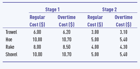
The cost of subcontracting in stage 1 adds 20% to the regular production cost.
The Spring Company wants to establish a production schedule for regular and overtime production in each stage and for the number of tool heads subcontracted, at the minimum cost. Formulate a linear programming model for this problem and solve the model using Excel. Which resources appear to be most critical in the production process?
Walsh's Juice Company
Walsh's Juice Company produces three products from unprocessed grape juice—bottled juice, frozen juice concentrate, and jelly. It purchases grape juice from three vineyards near the Great Lakes. The climate in this area is good for growing the concord grapes necessary to produce grape juice products. The grapes are harvested at the vineyards and immediately converted into juice at plants at the vineyard sites and stored in refrigerated tanks. The juice is then transported to four different plants in Virginia, Michigan, Tennessee, and Indiana, where it is processed into bottled grape juice, frozen concentrated juice, and jelly. Vineyard output typically differs each month in the harvesting season and the plants have different processing capacity.
In a particular month the vineyard in New York has 1400 tons of unprocessed grape juice available, while the vineyard in Ohio has 1700 tons and the vineyard in Pennsylvania has 1100 tons. The processing capacity per month is 1200 tons of unprocessed juice at the plant in Virginia, 1100 tons of juice at the plant in Michigan, 1400 tons at the plant in Tennessee, and 1400 tons at the plant in Indiana. The cost per ton of transporting unprocessed juice from the vineyards to the plant is as follows:
Vineyard | Plant | |||
|---|---|---|---|---|
Virginia | Michigan | Tennessee | Indiana | |
New York | $850 | 720 | 910 | 750 |
Pennsylvania | 970 | 790 | 1050 | 880 |
Ohio | 900 | 830 | 780 | 820 |
The plants are different ages, have different equipment, and have different wage rates; thus, the cost of processing each product at each plant ($/ton) differs as follows:
Vineyard | Plant | |||
|---|---|---|---|---|
Virginia | Michigan | Tennessee | Indiana | |
Juice | $2100 | 2350 | 2200 | 1900 |
Concentrate | 4100 | 4300 | 3950 | 3900 |
Jelly | 2600 | 2300 | 2500 | 2800 |
This month the company needs to process a total of 1200 tons of bottled juice, 900 tons of frozen concentrate, and 700 tons of jelly at the four plants combined. However, the production process for frozen concentrate results in some juice dehydration, and the process for jelly includes a cooking stage that evaporates water content. To process 1 ton of frozen concentrate requires 2 tons of unprocessed juice; a ton of jelly requires 1.5 tons of un-processed juice; and a ton of bottled juice requires 1 ton of unprocessed juice.
Walsh's management wants to determine how many tons of grape juice to ship from each of the vineyards to each of the plants, and the number of tons of each product to process at each plant. Thus, management needs a model that includes both the logistical aspects of this problem and the production processing aspects. It wants a solution that will minimize total costs, including the cost of transporting grape juice from the vineyards to the plants and the product processing costs. Help Walsh's solve this problem by formulating a linear programming model and solve it using Excel.
Julia's Food Booth
Julia Robertson is a senior at Tech, and she's investigating different ways to finance her final year at school. In her first three years at school she worked a part-time job at a local bar, but she wants more free time during the week in her senior year to interview for jobs after she graduates, to work on some senior projects, and to have some fun with her friends. She is considering leasing a food booth outside the stadium at the Tech home football games which Tech allows for selected students and student groups. Tech sells out every home game, and she knows from going to the games herself that everyone eats a lot of food. She has to pay $1000 per game for a booth and the booths are not very large. Vendors can sell only food or drinks on Tech property but not both. Only the Tech athletic department concession stands can sell both inside the stadium. She thinks slices of cheese pizza, hot dogs, and barbecue sandwiches are the most popular food items among fans, so these are the items she would sell.
Most food items are sold during the hour before the game starts and during half time; thus, it will not be possible for Julia to prepare the food while she is selling it. She must prepare the food ahead of time and then store it in a warming oven. She can lease a warming oven for the home season, which includes six games, for $600. The oven has 16 shelves, and each shelf is 3 ft by 4 ft. She plans to fill the oven with the three food items before the game and before half time.
Julia has negotiated with a local pizza delivery company to deliver 14-inch cheese pizzas twice each game; two hours before the game and right after the opening kickoff. Each pizza will cost her $6 and will include eight slices. She estimates it will cost her $0.45 for each hot dog and $0.90 for each barbecue sandwich if she makes the barbecue herself the night before. She measured a hot dog and found it takes up about 16 in.2 of space, while a barbecue sandwich takes up about 25 in.2 She plans to sell a slice of pizza and a hot dog for $1.50 apiece and a barbecue sandwich for $2.25. She has $1500 in cash available to purchase and prepare the food items for the first home game; for the remaining five games she will purchase her ingredients with money she has made from the previous game.
Julia has talked to some students and vendors who have sold food at previous football games at Tech as well as at other universities. From this she has discovered that she can expect to sell at least as many slices of pizza as hot dogs and barbecue sandwiches combined. She also anticipates that she will probably sell at least twice as many hot dogs as barbecue sandwiches. She believes that she will sell everything she can stock and develop a customer base for the season if she follows these general guidelines for demand.
If Julia clears at least $1000 in profit for each game after paying all her expenses, she believes it will be worth leasing the booth.
Formulate and solve a linear programming model for Julia that will help you advise her if she should lease the booth.
If Julia can borrow some more money from a friend before the first game to purchase more ingredients, could she increase her profit? If so, how much should she borrow and how much additional profit would she make? What factor constrains her from borrowing even more money than this amount (indicated in your answer to the previous question)?
When Julia looked at the solution in (a), she realized that it would be physically difficult for her to prepare all the hot dogs and barbecue sandwiches indicated in this solution. She believes she can hire a friend of hers to help her for $100 per game. Based on the results in (a) and (b), is this something you think she could reasonably do and should do?
Julia seems to be basing her analysis on "certain" assumptions that everything will go as she plans. What are some of the uncertain factors in the model that could go wrong and adversely affect Julia's analysis? Given these uncertainties and the results in (a), (b), and (c), what do you recommend that Julia do?
The Sea Village Amusement Park
Sea Village is a large amusement and water park located on the coast of South Carolina. The park hires high school and college students to work during the summer months of May, June, July, August, and September. The student employees operate virtually all of the highly mechanized, computerized rides; perform as entertainers; perform most of the custodial work during park hours; make up the work force for restaurants, food services, retail shops, and stores; drive trams; and park cars. Park management has assessed their monthly needs based on previous summers' attendance at the park, and the expected available work force. Park attendance is relatively low in May until public schools are out, then it increases through June, July, and August, and decreases dramatically in September when schools reopen after Labor Day. The park is open seven days a week through the summer until September when it cuts back to weekends only. Management estimates that it will require 21,000 hours of labor in each of the first two weeks of May, 26,000 hours during the third week of May, and 32,000 hours during the last week in May. During the first two weeks of June, it will require at least 36,000 hours of labor and 41,000 hours during the last two weeks in June. In July, 46,000 hours will be required each week, and in August 47,000 hours will be needed each week. In September, they will only need 14,000 hours in the first week, 12,000 hours in each of the second and third weeks, and 9,000 hours the last week of September.
The park hires new employees each week from the first week in May through August. A new employee mostly trains the first week by observing and helping more experienced employees; however, they do work approximately 10 hours under the supervision of an experienced employee. An employee is considered experienced after completing one week on the job. Experienced employees are considered part-time and are scheduled to work 30 hours per week in order to eliminate overtime and reduce the cost of benefits, and to give more students the opportunity to work. However, no one is ever laid off or will be scheduled for less (or more) than 30 hours, even if more employees are available than needed. Management believes this is a necessary condition of employment because so many of the student employees move to the area during the summer just to work in the park and live near the beach nearby. If these employees were sporadically laid off and were stuck with lease payments and other expenses, it would be bad public relations and hurt employment efforts in future summers. Although no one is laid off, 15% of all experienced employees quit each week for a variety of reasons, including homesickness, illness, and other personal reasons, plus some are asked to leave because of very poor job performance.
Park management is able to start the first week in May with 800 experienced employees who worked in the Park in previous summers and live in the area. They are generally able to work a lot of hours on the weekends and then some during the week; however, in May, attendance is much heavier on the weekend so most of the labor hours are needed then. The park expects to have a pool of 1,600 available applicants to hire for the first week in May. After the first week, the pool is diminished by the number of new employees hired the previous week, but each week through June the park gets 210 new job applicants, which decreases to 120 new applicants each week for the rest of the summer. For example, the available applicant pool in the second week in May would be the previous week's pool, which in week 1 is 1,600, minus the number of new employees hired in week 1, plus 210 new applicants. At the end of the last week in August, 75% of all the experienced employees will quit to go back to school and the park will not hire any new employees in September. The park must operate in September using experienced employees who live in the area, but the weekly attrition rate for these employees in September drops to 12%.
Formulate and solve a linear programming model to assist the park's management to plan and schedule the number of new employees it hires each week that will minimize the total number of new employees it must hire during the summer.
Charnes, A., and W. W. Cooper. Management Models and Industrial Applications of Linear Programming. New York: John Wiley & Sons, 1961.
Dantzig, G. B. Linear Programming and Extensions. Princeton, NJ: Princeton University, 1963.
Gass, S. Linear Programming, 4th ed. New York: McGraw-Hill, 1975.
Moore, L. J., S. M. Lee, and B. W. Taylor. Management Science, 4th ed. Needham Heights, MA: Allyn and Bacon, 1993.
Taylor, B. W. Introduction to Management Science, 6th ed. Upper Saddle River, NJ: Prentice Hall, 1999.
Wagner, A. M. Principles of Operations Research, 2nd ed. Upper Saddle River, NJ: Prentice Hall, 1975.