
In this chapter, you will learn about . . .
The Sales and Operations Planning Process
Strategies for Adjusting Capacity
Strategies for Managing Demand
Quantitative Techniques for Aggregate Planning
The Hierarchical Nature of Planning
Aggregate Planning for Services

Web resources for this chapter include
OM Tools Software
Internet Exercises
Online Practice Quizzes
Lecture Slides in PowerPoint
Virtual Tours
Excel Worksheets
Excel Exhibits
Company and Resource Weblinks
www.wiley.com/college/russell
Sales and Operations Planning AT HERSHEY'S
The seasonal demand for chocolate, coupled with its limited shelf life, requires careful coordination of sales and operations planning. Strategies for increasing demand may have unintended consequences for the bottom line if production capabilities and costs are not considered.
Since over 50% of candy purchases are impulse buys, product promotions and merchandising can have a dramatic influence on sales. For example, one way to generate new sales is to take a stable product like Hershey's kisses and dress it up for different seasons (red and green wrapper for Christmas, red and silver for Valentine's Day, pink and green for Easter), or create upscale versions for special occasions, such as chocolate mint, dark chocolate, or white chocolate hugs. However, while seasonal products may increase demand, without a corresponding increase in production of the "right" items and a revised distribution plan, product shortages or soaring production and supply chain costs may negate the increased revenue. Overforecasting demand can be problematic as well, resulting in obsolete inventories due to outdated seasons or expired shelf life.
To prevent these problems, companies use a systematic approach to matching supply and demand, called sales and operations planning (S&OP). At Hershey's, prior year results and trends, as well as promotional plans, are studied by a seasonal consensus team that develops sales estimates. These estimates are adjusted after customer planning meetings with key clients (such as Target or Walmart). Promotions and plan-ograms are designed, and customer replenishment plans are developed that take into account consumption, inventory, and service levels. These, in turn, are matched with factory shipment plans and an operations plan is developed. S&OP meetings between sales, operations, and finance on a weekly basis ensure that the plans are being executed properly and adjustments are made as necessary.
In this chapter we'll learn how companies, such as Hershey's, plan their resource levels to match supply and demand. We begin with a discussion of the nature of sales and operations planning (S&OP), then continue with strategies for managing demand and adjusting capacity. We conclude with a discussion of hierarchical planning decisions, collaborative planning with trading partners, and aggregate planning for services.
Sources: Adapted from Ameer Ali and Herb Hockley, "Hershey Foods: Sweet Results with SAP Demand Planning," SAPPHIRE 2008: Orlando (May, 2008), retrieved from htto://www.sap.com/community/showdetail.epx?itemID=11738; and Nick Rosekelly, "Seasonal Products: Identifying Long-Term Potential with Short-Term Trial," Stagnito's New Products Magazine (May 2003), retrieved from http://www.allbusiness.com/business-planning-structures/starting-a-business/152936-1.html.
Sales and operations planning (S&OP): a process for coordinating supply and demand.
Sales and Operations Planning (S&OP) is an aggregate planning process that determines the resource capacity a firm will need to meet its demand over an intermediate time horizon—6 to 12 months in the future. Within this time frame, it is usually not feasible to increase capacity by building new facilities or purchasing new equipment; however, it is feasible to hire or lay off workers, increase or reduce the workweek, add an extra shift, subcontract out work, use overtime, or build up and deplete inventory levels.
Aggregate refers to sales and operations planning for product lines or families.
We use the term aggregate because the plans are developed for product lines or product families, rather than individual products. An aggregate operations plan might specify how many bicycles are to be produced but would not identify them by color, size, tires, or type of brakes. Resource capacity is also expressed in aggregate terms, typically as labor or machine hours. Labor hours would not be specified by type of labor, nor machine hours by type of machine. And they may be given only for critical processes.
For services, capacity is often limited by space—number of airline seats, number of hotel rooms, number of beds in a correctional facility. Time can also affect capacity. The number of customers who can be served lunch in a restaurant is limited by the number of seats, as well as the number of hours lunch is served. In some overcrowded schools, lunch begins at 10:00 a.m. so that all students can be served by 2:00 p.m.!

Producers of pulp, paper, lumber, and other wood products have an interesting aggregate planning problem—they must plan for the renewable resource of trees. Aggregate planning starts with a mathematical simulation model of tree growth that determines the maximum sustainable flow of wood fiber from each acreage. Decisions are made as to which trees to harvest now; which ones to leave until later; where to plant new trees; and the type, amount, and location of new timberland that should be purchased. The planning horizon is the biological lead time to grow trees—more than 80 years!
There are two objectives to sales and operations planning:
To establish a company-wide game plan for allocating resources, and
To develop an economic strategy for meeting demand.
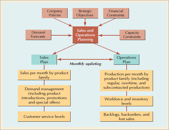
The first objective refers to the long-standing battle between the sales and operations functions within a firm. Personnel who are evaluated solely on sales volume have the tendency to make unrealistic sales commitments (either in terms of quantity or timing) that operations is expected to meet, sometimes at an exorbitant price. Operations personnel who are evaluated on keeping manufacturing costs down may refuse to accept orders that require additional financial resources (such as overtime wage rates) or hard-to-meet completion dates. The job of operations planning is to match forecasted demand with available capacity. If capacity is inadequate, it can usually be expanded, but at a cost. The company needs to determine if the extra cost is worth the increased revenue from the sale, and if the sale is consistent with the strategy of the firm. Thus, the aggregate plan should not be determined by manufacturing personnel alone; rather, it should be agreed on by top management from all the functional areas of the firm—operations, marketing, and finance. Because this is such an important decision, companies engage in a structured, collaborative decisionmaking process called sales and operations planning (S&OP). Figure 14.1 outlines the S&OP process.
As shown in Figure 14.l, the sales and operations plan should reflect company policy (such as avoiding layoffs, limiting inventory levels, and maintaining a specified customer service level) and strategic objectives (such as capturing a certain share of the market or achieving targeted levels of quality or profit). Other inputs include financial constraints, demand forecasts (from sales), and capacity constraints (from operations).
Given these inputs, the sales function develops a monthly sales plan. A forecasting model is run to create preliminary demand figures, then adjusted based on input from key customers and sales personnel in the field. The forecast is further adjusted for planned promotions, product introductions, and special offers. Finally, a customer service level is set which specifies the percent of customer demand that should be satisfied.
The sales plan is then shared with the operations function that must convert the sales to production requirements as economically as possible. Operations develops a schedule of production per month by product family that includes the number of workers and other resources needed, and whether the production plan requires overtime or subcontracting. The production plan also shows the anticipated inventory levels, backlog (work not yet completed), backorders (work performed later for customers willing to wait for their order), and lost sales (customers whose orders could not be completed or were not accepted).
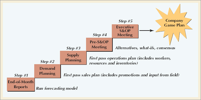
The sales and operations planning process does not stop here. The two plans must be reconciled. Typically this involves creating an annual plan and updating it with monthly meetings that culminate in executive approval of the final plan. The process is diagrammed in Figure 14.2.
Because of the various factors and viewpoints considered, the sales and operations plan is often referred to as the company's game plan for the coming year, and deviations from the plan are carefully monitored. Monthly S&OP meeting reconcile differences in supply, demand, and new product plans.
An economic strategy for meeting demand can be attained by either adjusting capacity or managing demand. We discuss both approaches in the following sections. Please note that the terms operations plan, production plan, and aggregate plan are used interchangeably in this text book.
A LONG THE SUPPLY CHAIN
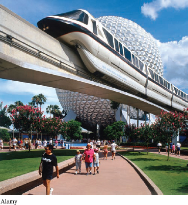
Sales and operations planning at Disney World is all about people—how many people visit the parks and what they do while there. The Disney property in Florida includes 4 parks, 20 hotels, 27,500 rooms, 160 miles of roads, and 56,000 employees. Forecasting attendance and guest behavior helps plan for more than 1 billion customer interactions per year, and the purchase of 9 million hamburgers, 50 million Cokes, and tons of "tangible memories."
Planning begins with a five-year forecast of attendance based on a combination of econometric models, experiencebased models, extensive research, and a magic mirror. The econometric model examines the international economies of seven key countries, their GDP growth, foreign exchange rate, and consumer confidence. The experience-based model looks at demographics, planned product introductions, capacity expansions, and marketing strategies. Extensive research is conducted by 35 analysts and 70 field personnel year round. Over 1 million surveys are administered to key household segments, current guests, cast members, and travel industry personnel. The magic mirror is the patented part of the forecasting procedure that, in part, accounts for the mere 5% error in the five-year attendance forecast and the 0% error in annual forecasts.
Disney's five-year plan is converted to an annual operating plan (AOP) for each park. Demand is highly seasonal and varies by month and day of the week. Economic conditions affect annual plans, as do history and holidays, school calendars, societal behavior, and sales promotions. The AOP is updated monthly with information from airline specials, hotel bookings, recent forecast accuracies, Web site monitoring, and competitive influences. A daily forecast of attendance is made by tweaking the AOP and adjusting for monthly variations, weather forecasts, and the previous day's crowds. Attendance drives all other decisions.
Disney is a master at adjusting its capacity and managing its demand. Capacity can be increased by lengthening park hours, opening more rides or shows, adding roving food and beverage carts, and deploying more "cast members." Demand is managed by limiting access to the park, shifting crowds to street activities, and taking reservations for attractions (ever used a fast pass?). Operating standards strictly regulate when these actions are taken. Obsessive collection of data ensures the response is timely.
Parks generally open at 9:00 a.m. each day, but an unusually high count of 7:30 a.m. breakfast patrons at on-property hotels will prompt early openings at select locations. By 11:00 a.m. the day's attendance forecast is updated based on traffic, the weather, entry patterns, and crowds at key attractions. The daily operating plan is continually updated every 20 minutes throughout the day from data collected by cast members using handheld computers. To maintain flexibility, cast members are scheduled in 15-minute intervals at various jobs throughout the park.
For Disney, pleasing the customer and making a profit takes careful planning. What other types of industries could benefit from a flexible planning process such as Disney's?
Source: Joni Newkirk and Mark Haskell, "Forecasting in the Service Sector," Presented at the Twelfth Annual Meeting of the Production Operations Management Society, Orlando, FL, April 1, 2001.
Disney is a master at forecasting aggregate demand for its theme parks, as well as adjusting capacity in time increments as small as 15 minutes.
Aggregate planning evaluates alternative capacity sources to find an economic strategy for satisfying demand.
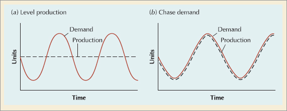
If demand for a company's products or services is stable over time, then the resources necessary to meet demand are acquired and maintained over the time horizon of the plan, and minor variations in demand are handled with overtime or undertime. Aggregate planning becomes more of a challenge when demand fluctuates over the planning horizon. For example, seasonal demand patterns can be met by:
Producing at a constant rate and using inventory to absorb fluctuations in demand (level production)
Maintaining resources for high-demand levels
Increasing or decreasing working hours (overtime and undertime)
Subcontracting work to other firms
Using part-time workers
Providing the service or product at a later time period (backordering)
When one of these alternatives is selected, a company is said to have a pure strategy for meeting demand. When two or more are selected, a company has a mixed strategy.
• Pure strategy: adjusting only one capacity factor to meet demand.
• Level production: producing at a constant rate and using inventory as needed to meet demand.
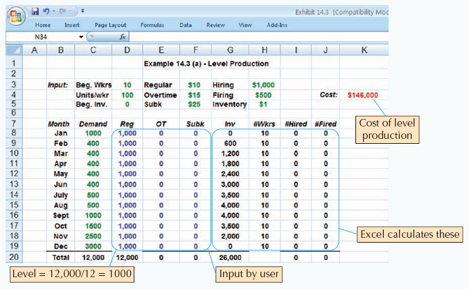
The level production strategy, shown in Figure 14.3a, sets production at a fixed rate (usually to meet average demand) and uses inventory to absorb variations in demand. During periods of low demand, overproduction is stored as inventory, to be depleted in periods of high demand. The cost of this strategy is the cost of holding inventory, including the cost of obsolete or perishable items that may have to be discarded.
• Chase demand: changing workforce levels so that production matches demand.
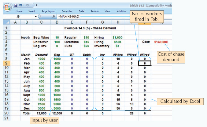
The chase demand strategy, shown in Figure 14.3b, matches the production plan to the demand pattern and absorbs variations in demand by hiring and firing workers. During periods of low demand, production is cut back and workers are laid off. During periods of high demand, production is increased and additional workers are hired. The cost of this strategy is the cost of hiring and firing workers. This approach would not work for industries in which worker skills are scarce or competition for labor is intense, but it can be quite cost-effective during periods of high unemployment or for industries with low-skilled workers.
A variation of chase demand is chase supply. For some industries, the production planning task revolves around the supply of raw materials, not the demand pattern. Consider Motts, the applesauce manufacturer, whose raw material is available only 40 days during a year. The work-force size at its peak is 1500 workers, but it normally consists of around 350 workers. Almost 10% of the company's payroll is made up of unemployment benefits—the price of doing business in that particular industry.
Maintaining resources for peak demand levels ensures high levels of customer service but can be very costly in terms of the investment in extra workers and machines that remain idle during low-demand periods. This strategy is used when superior customer service is important (such as Nordstrom's department store) or when customers are willing to pay extra for the availability of critical staff or equipment. Professional services trying to generate more demand may keep staff levels high, defense contractors may be paid to keep extra capacity "available," childcare facilities may elect to maintain staff levels for continuity when attendance is low, and full-service hospitals may invest in specialized equipment that is rarely used but is critical for the care of a small number of patients.
• Peak demand: staffing for high levels of customer service.
Overtime and undertime are common strategies when demand fluctuations are not extreme. A competent staff is maintained, hiring and firing costs are avoided, and demand is met temporarily without investing in permanent resources. Disadvantages include the premium paid for overtime work, a tired and potentially less efficient workforce, and the possibility that overtime alone may be insufficient to meet peak demand periods.
Overtime and undertime adjust working hours to meet demand.
Undertime can be achieved by working fewer hours during the day or fewer days per week. In addition, vacation time can be scheduled during months of slow demand. For example, furniture manufacturers typically shut down the entire month of July, while shipbuilding goes dormant in December. During the recent recession, 35% of U.S. employers surveyed used unpaid furloughs in lieu of more layoffs to adjust to decreased demand. Europe routinely uses shorter workweeks and mandatory vacations in economic downturns.
Subcontracting or outsourcing is a feasible alternative if a supplier can reliably meet quality and time requirements. This is a common solution for component parts when demand exceeds expectations for the final product. The subcontracting decision requires maintaining strong ties with possible subcontractors and first-hand knowledge of their work. Disadvantages of subcontracting include reduced profits, loss of control over production, long lead times, and the potential that the subcontractor may become a future competitor.
Subcontracting lets outside companies complete the work.
Using part-time workers is feasible for unskilled jobs or in areas with large temporary labor pools (such as students, homemakers, or retirees). Part-time workers are less costly than full-time workers—they receive no health-care or retirement benefits—and are more flexible—their hours usually vary considerably. Part-time workers have been the mainstay of retail, fast-food, and other services for some time and are becoming more accepted in manufacturing and government jobs. Japanese manufacturers traditionally use a large percentage of part-time or temporary workers. Part-time and temporary workers now account for one-third of our nation's workforce, and are expected to increase as companies gingerly enter recovery from the recession.
• Backlog: accumulated customer orders to be completed at a later date.
• Backordering: ordering an item that is temporarily out-of-stock.
• Lost sales: forfeited sales for out-of-stock items.
Companies that offer customized products and services accept customer orders and fill them at a later date. The accumulation of these orders creates a backlog that grows during periods of high demand and is depleted during periods of low demand. The planned backlog is an important part of the aggregate plan. For make-to-stock companies, customers who request an item that is temporarily out-of-stock may have the option of backordering the item. If the customer is unwilling to wait for the backordered item, the sale will be lost. Although in general both backorders and lost sales should be avoided, the aggregate plan may include an estimate of both. Backorders are added to the next period's requirements; lost sales are not.
Aggregate planning can also involve proactive demand management. Strategies for managing demand include:
Winter coat specials in July, bathing-suit sales in January, early-bird discounts on dinner, lower long-distance rates in the evenings, and getaway weekends at hotels during the off-season are all attempts to shift demand into different time periods. Electric utilities are especially skilled at off-peak pricing. Promotions can also be used to extend high demand into low-demand seasons. Holiday gift buying is encouraged earlier each year, and beach resorts plan festivals in September and October to extend the season. Successful demand management depends on accurate forecasts of demand and accurate forecasts of the changes in demand brought about by sales, promotions, and special offers.
Shift demand into other time periods.
Create demand for idle resources.
For industries with extreme variations in demand, offering products or services with countercyclical demand patterns helps smooth out resource requirements. This approach involves examining the idleness of resources and creating a demand for those resources. McDonald's offers breakfast to keep its kitchens busy during the prelunch hours, pancake restaurants serve lunch and dinner, and heating firms also sell air conditioners.
Amadas Industries, a small U.S. manufacturer of peanut harvesting equipment, does an especially good job of finding countercyclical products to smooth the load on its manufacturing facilities. The company operates a job shop production system with general-purpose equipment, 50 highly skilled workers, and a talented engineering staff. With these flexible resources, the company can make virtually anything its engineers can design. Inventories of finished goods are limited because of the significant investment in funds and the size of the finished product. Demand for the product is highly seasonal. Peanut-harvesting equipment is generally purchased on an as-needed basis from August to October, so during the spring and early summer, the company makes bark-scalping equipment for processing mulch and pine nuggets used by landscaping services. Demand for peanut-harvesting equipment is also affected by the weather each growing season, so during years of extensive drought, the company produces and sells irrigation equipment. The company also decided to market its products internationally with a special eye toward countries whose growing seasons are opposite to that of the United States. Thus, many of its sales are made in China and India during the very months when demand in the United States is low.
Another approach to managing demand recognizes the information distortion caused by ordering goods in batches along a supply chain. Even though a customer may require daily usage of an item, he or she probably does not purchase that item daily. Neither do retail stores restock their shelves continuously. By the time a replenishment order reaches distributors, wholesalers, manufacturers, and their suppliers, the demand pattern for a product can appear extremely erratic. This bullwhip effect was discussed in Chapter 10. To control the situation, manufacturers, their suppliers, and customers form partnerships in which demand information is shared and orders are placed in a more continuous fashion.
Share information along the supply chain.
A carefully planned mix of services can smooth out resource requirements. At this resort, the pristine golf course during the summer months becomes a cross-country skiing path during the winter. The same company that maintains the fairways, grooms the snow for the skiers.

• Aggregate planning: the process of determining the quantity and timing of production over an intermediate time frame.
One aggregate planning strategy is not always preferable to another. The most effective strategy depends on the demand distribution, competitive position, and cost structure of a firm or product line. Several quantitative techniques are available to help with the aggregate planning decision. In the sections that follow, we discuss pure and mixed strategies, linear programming, the transportation method, and other quantitative techniques.
Solving aggregate planning problems involves formulating strategies for meeting demand, constructing production plans from those strategies, determining the cost and feasibility of each plan, and selecting the lowest cost plan from among the feasible alternatives. The effectiveness of the aggregate planning process is directly related to management's understanding of the cost variables involved and the reasonableness of the scenarios tested. Example 14.1 compares the cost of two pure strategies: level production and chase demand.
• Pure strategy: varying only one capacity variable in aggregate planning.
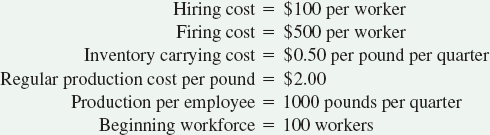
Aggregate Planning Using Pure Strategies
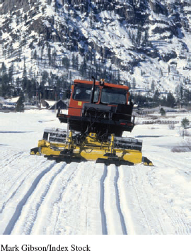
The Good and Rich Candy Company makes a variety of candies in three factories worldwide. Its line of chocolate candies exhibits a highly seasonal demand pattern, with peaks during the winter months (for the holiday season and Valentine's Day) and valleys during the summer months (when chocolate tends to melt and customers are watching their weight). Given the following costs and quarterly sales forecasts, determine whether (a) level production, or (b) chase demand would more economically meet the demand for chocolate candies:
Quarter | Sales Forecast (lbs) |
|---|---|
Spring | 80,000 |
Summer | 50,000 |
Fall | 120,000 |
Winter | 150,000 |
Solution
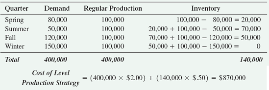
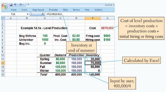
For the level production strategy, we first need to calculate average quarterly demand.

This becomes our planned production for each quarter. Since each worker can produce 1000 pounds a quarter, 100 workers will be needed each quarter to meet the production requirements of 100,000 pounds. Production in excess of demand is stored in inventory, where it remains until it is used to meet demand in a later period. Demand in excess of production is met by using inventory from the previous quarter. The production plan and resulting inventory costs are as follows:
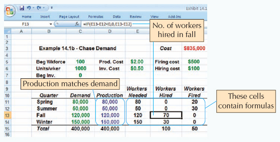
For the chase demand strategy, production each quarter matches demand. To accomplish this, workers are hired at a cost of $100 each and fired at a cost of $500 each. Since each worker can produce 1000 pounds per quarter, we divide the quarterly sales forecast by 1000 to determine the required workforce size each quarter. We begin with 100 workers and hire and fire as needed. The production plan and resulting hiring and firing costs are given here.
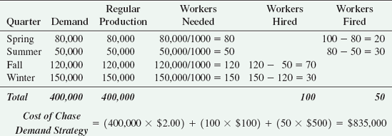
Comparing the cost of level production with chase demand, we find that chase demand is the best strategy for the Good and Rich line of candies.
The problem can also be solved using Excel. Exhibit 14.1 shows two worksheets from the Excel file, Exhibit 14.1.xls, available on the text Web site.
Although chase demand is the better strategy for Good and Rich from an economic point of view, it may seem unduly harsh on the company's workforce. An example of a good "fit" between a company's chase demand strategy and the needs of the workforce is Hershey's, located in rural Pennsylvania, with a demand and cost structure much like that of Good and Rich. The location of the manufacturing facility is essential to the effectiveness of the company's production plan. During the winter, when demand for chocolate is high, the company hires farmers from surrounding areas, who are idle at that time of year. The farmers are let go during the spring and summer, when they are anxious to return to their fields and the demand for chocolate falls. The plan is cost-effective, and the extra help is content with the sporadic hiring and firing practices of the company.
Au: Shifting of this para before next section is not possible, because it affect the pagination of whole chapter. Please suggest.
Linear programming gives an optimal solution, but demand and costs must be linear.
Strategies for production planning may be easy to evaluate, but they do not necessarily provide an optimal solution. Consider the Good and Rich Company of Example 14.1. The optimal production plan is probably some combination of inventory and workforce adjustment. We could simply try different combinations and compare the costs (i.e., the trial-and-error approach), or we could find the optimal solution by using linear programming. If you are unfamiliar with linear programming, please review the supplement to this chapter. Example 14.2 develops an optimal production plan for Good and Rich chocolate candies using linear programming.
Production Planning Using Linear Programming
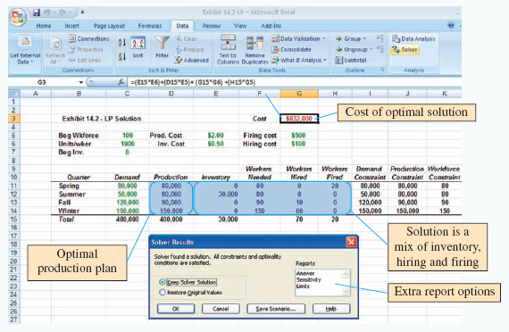
Formulate a linear programming model for Example 14.1 that will satisfy demand for Good and Rich chocolate candies at minimum cost. Solve the model with Excel Solver.
Solution
Model Formulation:
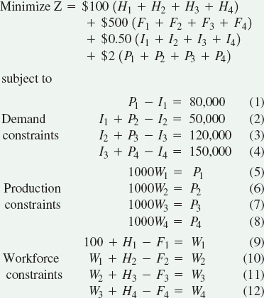
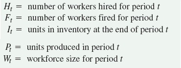
Objective function: The objective function seeks to minimize the cost of hiring workers, firing workers, holding inventory, and production. Cost values are provided in the problem statement for Example 14.1. The number of workers hired and fired each quarter and the amount of inventory held are variables whose values are determined by solving the linear programming (LP) problem.
Demand constraints: The first set of constraints ensures that demand is met each quarter. Demand can be met from production in the current period and inventory from the previous period. Units produced in excess of demand remain in inventory at the end of the period. In general form, the demand equations are constructed as
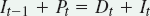
where Dt is the demand in period t, as specified in the problem. Leaving demand on the right-hand side, we have
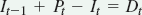
There are four demand constraints, one for each quarter. Since there is no beginning inventory, I0 = 0, and it can be dropped from the first demand constraint.
Production constraints: The four production constraints convert the workforce size to the number of units that can be produced. Each worker can produce 1000 units a quarter, so the production each quarter is 1000 times the number of workers employed, or

Workforce constraints: The workforce constraints limit the workforce size in each period to the previous period's workforce plus the number of workers hired in the current period minus the number of workers fired.
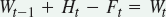
Notice the first workforce constraint shows a beginning workforce size of 100.
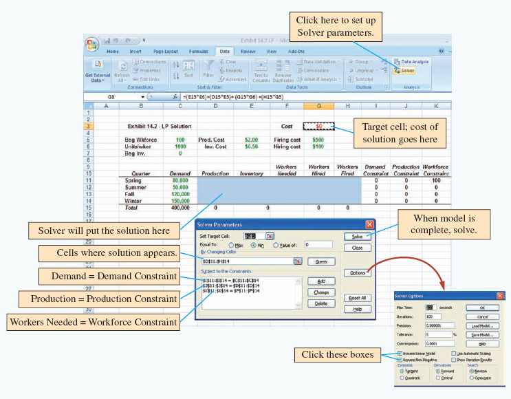
Additional variables and constraints: Additional variables, such as overtime and subcontracting, can be added to the LP formulation as needed. The cost of those variables is then added to the objective function. Additional constraints such as limiting the amount of overtime or subcontracting can also be added in the Solver model.
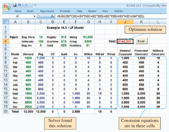
The LP formulation is solved using Excel Solver as shown in Exhibit 14.2b. The Excel file, Exhibit 14.2.xls, is available on the text Web site. The cost of the optimum solution is $832,000, an improvement of $3000 over the chase demand strategy and $38,000 over the level production strategy.
Most companies use mixed strategies for production planning. Mixed strategies can incorporate management policies, such as "no more than x% of the workforce can be laid off in one quarter" or "inventory levels cannot exceed x dollars." They can also be adapted to the quirks of a company or industry. For example, many industries that experience a slowdown during part of the year may simply shut down manufacturing during the low-demand season and schedule employee vacations during that time.
• Mixed strategy: varying two or more capacity factors to determine a feasible production plan.
Example 14.3 compares pure and mixed strategies in a more extensive aggregate planning problem. Excel spreadsheets are used to make the calculations. The user inputs demand and cost data, as well as values for regular, overtime, and subcontracted production. The spreadsheet calculates resulting inventory levels, workforce levels, hiring/firing and total cost. The Excel file for this example, Exhibit 14.3.xls is available on the textbook Web site. Although this problem can be solved by hand, you may wish to use the spreadsheet as a template for solving other aggregate planning problems.
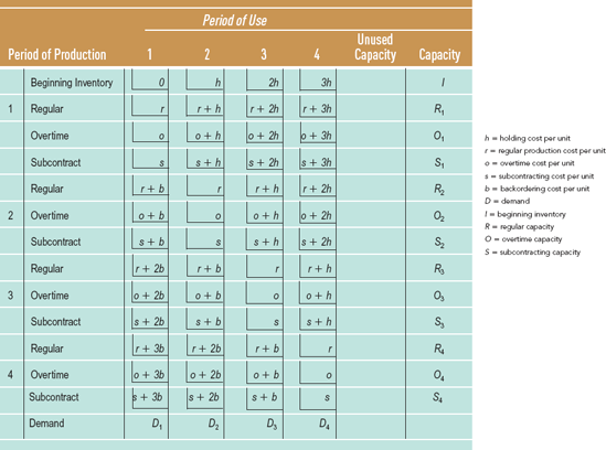
For cases in which the decision to change the size of the workforce has already been made or is prohibited, the transportation method of linear programming can be used to develop an aggregate production plan. (See Supplement 10 for an introduction to the transportation method.) The transportation method gathers all the cost information into one matrix and plans production based on the lowest-cost alternatives. Table 14.1 shows a blank transportation tableau with i for inventory, h for holding cost, r for regular production cost, o for overtime, s for subcontracting, and b for backordering. The capital letters indicate individual capacities or demand. The periods of production, along with the production options, appear in the first column. The periods of use (regardless of when the items are produced) appear across the top row. Cost entries in the period-of-use columns differ by the cost of holding the item in inventory before its use.
Use the transportation method when hiring and firing is not an option.
Example 14.4 illustrates the transportation method of aggregate planning. A blank transportation tableau and an Excel file of Example 14.4 are available online.
Although linear programming models will yield an optimal solution to the aggregate planning problem, there are some limitations. The relationships among variables must be linear, the model is deterministic, and only one objective is allowed (usually minimizing cost).
The linear decision rule, search decision rule, and management coefficients model use different types of cost functions to solve aggregate planning problems. The linear decision rule (LDR) is an optimizing technique originally developed for aggregate planning in a paint factory. It solves a set of four quadratic equations that describe the major capacity-related costs in the factory: payroll costs, hiring and firing, overtime and undertime, and inventory costs. The results yield the optimal workforce level and production rate.
Linear decision rule (LDR): a mathematical technique for aggregate planning.
The search decision rule (SDR) is a pattern search algorithm that tries to find the minimum cost combination of various workforce levels and production rates. Any type of cost function can be used. The search is performed by computer and may involve the evaluation of thousands of possible solutions, but an optimal solution is not guaranteed. The management coefficients model uses regression analysis to improve the consistency of planning decisions. Techniques like SDR and management coefficients are often embedded in commercial decision support systems or expert systems for aggregate planning.
• Search decision rule (SDR): a pattern search technique for aggregate planning.
The Transportation Method of Aggregate Planning
Burruss Manufacturing Company uses overtime, inventory, and subcontracting to absorb fluctuations in demand. An aggregate production plan is devised annually and updated quarterly. Cost data, expected demand, and available capacities in units for the next four quarters are given here. Demand must be satisfied in the period it occurs; that is, no backordering is allowed. Design a production plan that will satisfy demand at minimum cost.
Quarter | Expected Demand | Regular Capacity | Overtime Capacity | Subcontract Capacity |
|---|---|---|---|---|
1 | 900 | 1000 | 100 | 500 |
2 | 1500 | 1200 | 150 | 500 |
3 | 1600 | 1300 | 200 | 500 |
4 | 3000 | 1300 | 200 | 500 |
Regular production cost per unit $20
Overtime production cost per unit $25
Subcontracting cost per unit $28
Inventory holding cost per unit per period $ 3
Beginning inventory 300 units
Solution
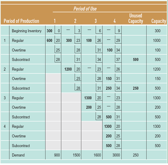
The problem is solved using the transportation tableau shown in Table 14.2. The tableau is a worksheet that is completed as follows:
Rim Requirements
To set up the tableau, demand requirements for each quarter are listed on the bottom row, and capacity constraints for each type of production (i.e., regular, overtime, or subcontracting) are placed in the far right column.

Next, cost figures are entered into the small square at the corner of each cell. Starting with the beginning inventory row, inventory on hand in period 1 that is used in period 1 incurs zero cost. Inventory on hand in period 1 that is not used until period 2 incurs a $3 holding cost. Inventory held until period 3, costs $3 more, or $6. Similarly, inventory held until period 4 costs an additional $3, or $9.
Beginning Inventory
For regular production, a unit produced in period 1 and used in period 1, costs $20. A unit produced under regular production in period 1 but not used until period 2, incurs a production cost of $20 plus an inventory cost of $3, or $23. If the unit is held until period 3, it costs $3 more, or $26. If held until period 4, it costs $29. The cost calculations continue for overtime and subcontracting, beginning with production costs of $25 and $28, respectively.
Cost figures
The costs for production in periods 2, 3, and 4 are determined in a similar fashion, with one exception. Half of the remaining transportation tableau is blocked out as infeasible. This occurs because no backordering is allowed for this problem, and production cannot take place in one period to satisfy demand for a period that has already passed.
No backorders
Now that the tableau is set up, we can begin to allocate units to the cells and develop our production plan. The procedure is to assign units to the lowest-cost cells in a column so that demand requirements for the column are met, yet capacity constraints of each row are not exceeded. Beginning with the first demand column for period 1, we have 300 units of beginning inventory available to us at no cost. If we use all 300 units in period 1, there is no inventory left for use in later periods. We indicate this fact by putting a dash in the remaining cells of the beginning inventory row. We can satisfy the remaining 600 units of demand for period 1 with regular production at a cost of $20 per unit.
Allocating units to cells: Period 1
In period 2, the lowest-cost alternative is regular production in period 2. We assign 1200 units to that cell and, in the process, use up all the capacity for that row. Dashes are placed in the remaining cells of the row to indicate that they are no longer feasible choices. The remaining units needed to meet demand in period 2 are taken from regular production in period 1 that is inventoried until period 2, at a cost of $23 per unit. We assign 300 units to that cell.
Period 2
Continuing to the third period's demand of 1600 units, we fully utilize the 1300 units available from regular production in the same period and 200 units of overtime production. The remaining 100 units are produced with regular production in period 1 and held until period 3, at a cost of $26 per unit. As noted by the dashed line, period 1's regular production has reached its capacity and is no longer an alternative source of production.
Period 3
Of the fourth period's demand of 3000 units, 1300 units come from regular production, 200 from overtime, and 500 from subcontracting in the same period. One hundred fifty more units can be provided at a cost of $31 per unit from overtime production in period 2 and 500 from subcontracting in period 3. The next-lowest alternative is $34 from overtime in period 1 or subcontracting in period 2. At this point, we can make a judgment call as to whether our workers want overtime or whether it would be easier to subcontract out the entire amount. As shown in Table 14.2, we decide to use overtime to its full capacity of 100 units and fill the remaining demand of 250 from subcontracting.
Period 4
The unused capacity column is filled in last. In period 2, 250 units of subcontracting capacity are available but unused. This information is valuable because it tells us the flexibility the company has to accept additional orders.
Unused capacity
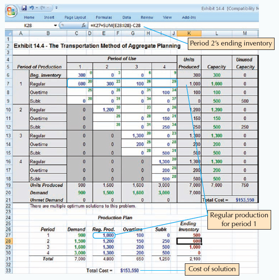
The optimal production plan, derived from the transportation tableau, is given in Table 14.3.[20] The values in the production plan are taken from the transportation tableau one row at a time.
The Production Plan
Table 14.3. The Production Plan
Period | Demand | Production Plan | |||
|---|---|---|---|---|---|
Regular Production | Overtime | Subcontract | Ending Inventory | ||
1 | 900 | 1000 | 100 | 0 | 500 |
2 | 1500 | 1200 | 150 | 250 | 600 |
3 | 1600 | 1300 | 200 | 500 | 1000 |
4 | 3000 | 1300 | 200 | 500 | 0 |
Total | 7000 | 4800 | 650 | 1250 | 2100 |
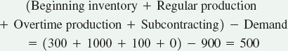
For example, the 1000 units of a regular production for period 1 is the sum of 600 + 300 + 100 from the second row of the transportation tableau. Ending inventory is calculated by summing beginning inventory, and all forms of production for that period and then subtracting demand. For example, the ending inventory for period 1 is
The cost of the production plan can be determined directly from the transportation tableau by multiplying the units in each cell times the cost in the corner of the cell and summing them. Alternatively, the cost can be determined from the production plan by multiplying the total units produced in each production category, or held in inventory, by their respective costs and summing them, as follows:
Cost of the plan
An Excel solution to this problem is shown in Exhibit 14.4.
• Management coefficients model: a regression techniques for aggregate planning
Planning involves a hierarchy of decisions. By determining a strategy for meeting and managing demand, aggregate planning provides a framework within which shorter term production and capacity decisions can be made. The levels of production and capacity planning are shown in Figure 14.4. In production planning, the next level of detail is a master production schedule, in which weekly (not monthly or quarterly) production plans are specified by individual final product (not product line). At another level of detail, material requirements planning plans the production of the components that go into the final products. Shop floor scheduling schedules the manufacturing operations required to make each component.
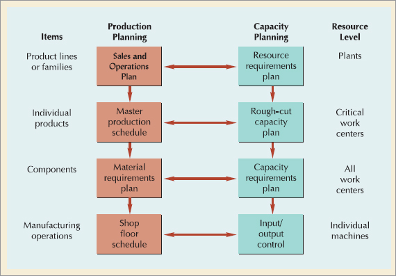
In capacity planning, we might develop a resource requirements plan, to verify that a sales and operations plan is doable, and a rough-cut capacity plan as a quick check to see if the master production schedule is feasible. One level down, we would develop a much more detailed capacity requirements plan that matches the factory's machine and labor resources to the material requirements plan. Finally, we would use input/output control to monitor the production that takes place at individual machines or work centers.
At each level, decisions are made within the parameters set by the higher-level decisions. The process of moving from the aggregate plan to the next level down is called disaggregation. We examine this process more thoroughly in Chapter 15. In the next section, we discuss two important tools for planning in an e-business environment: collaborative planning and available-to-promise.
• Disaggregation: the process of breaking an aggregate plan into more detailed plans.
• Collaborative planning: sharing information and synchronizing production across the supply chain.
Collaborative planning is part of the supply chain process of collaborative planning, forecasting, and replenishment (CPFR) presented in Chapter 10. In terms of production, CPFR involves selecting the products to be jointly managed, creating a single forecast of customer demand, and synchronizing production across the supply chain. Consensus among partners is reached first on the sales forecast, then on the production plan. Although the process differs by software vendor, basically each partner has access to an Internet-enabled planning book in which forecasts, customer orders, and production plans are visible for specific items. Partners agree on the level of aggregation to be used. Events trigger responses by partners. Alerts warn partners of conditions that require special action or changes to the plan.
One example of an event that requires collaboration among trading partners is quoting available-to-promise dates for customers.
In the current business environment of outsourcing and build-to-order products, companies must be able to provide the customer with accurate promise dates. Recall that S&OP is the company's game plan for matching supply and demand. As the time horizon grows shorter and more information becomes available, we develop and execute more detailed plans of action. For example, we convert the sales and operations plan for product families into a master schedule for individual products based on best estimates of future demand. As customer orders come in consuming the forecast, the remaining quantities are available-to-promise to future customers. Example 14.5 illustrates the process.
• Available-to-promise (ATP): the quantity of items that can be promised to the customer; the difference between planned production and customer orders already received.
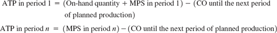
Available-to-promise is the difference between customer orders (CO) and planned production. In the first period of the planning horizon, available-to-promise is calculated by summing the on-hand quantity and planned production, then subtracting customer orders up until the next period of planned production. In subsequent periods, the ATP is simply planned production minus customer orders. No on-hand quantities are used. However, if customer orders exceed production, units can be taken from the ATP of previous periods.
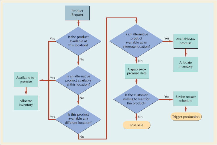
As companies venture beyond their boundaries to complete customer orders, so available-to-promise inquiries extend beyond a particular plant or distribution center to a network of plants and supplier's plants worldwide. ATP may also involve drilling down beyond the end item level to check the availability of critical components. Supply chain and enterprise planning software vendors such as SAP and i2 have available-to-promise modules that execute a series of rules when assessing product availability, and alert the planner when customer orders exceed or fall short of forecasts. The rules prescribe product substitutions, alternative sources, and allocation procedures as shown in Figure 14.5. When the product is not available, the system proposes a capable-to-promise date that is subject to customer approval.
• Capable-to-promise: the quantity of items that can be produced and made available at a later date.
Available-to-Promise
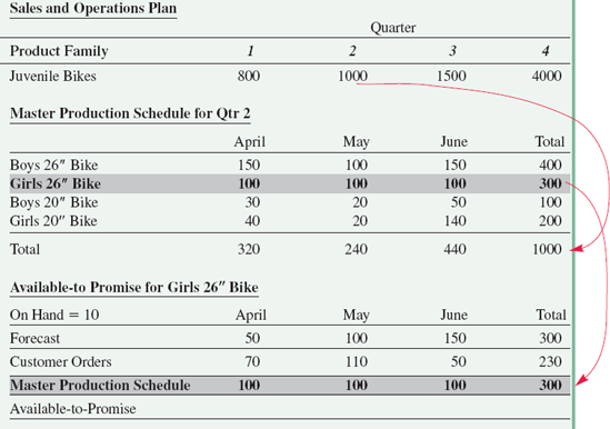
East Coast Bicycle Company has recently begun to accept customer orders over the Internet. The company uses both an aggregate production plan for families and a master production schedule for individual products. Now East Coast wants to add available-to-promise functionality to the planning process. Using the information given below, determine how many girls 26" bikes are available-to-promise in April, May, and June.
Solution
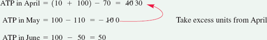
The available-to-promise (ATP) row is calculated by summing the on-hand quantity with the scheduled production units and subtracting the customer orders up until the next period of planned production. The negative ATP in May is offset by using 10 units of ATP from April.
On Hand = 10 | April | May | June |
Forecast | 50 | 100 | 150 |
Customer Orders | 70 | 110 | 150 |
Master Production Schedule | 100 | 100 | 100 |
Available-to-Promise | 30 | 0 |
Characteristics of aggregate planning for services
The aggregate planning process is different for services in the following ways:
Most services cannot be inventoried. It is impossible to store an airline seat, hotel room, or hair appointment for use later when demand may be higher. When the goods that accompany a service can be inventoried, they typically have a very short life. Newspapers are good for only a day; flowers, at most a week; and cooked hamburgers, only 10 minutes.
Demand for services is difficult to predict. Demand variations occur frequently and are often severe. The exponential distribution is commonly used to simulate the erratic demand for services—high-demand peaks over short periods of time with long periods of low demand in between. Customer service levels established by management express the percentage of demand that must be met and, sometimes, how quickly demand must be met. This is an important input to aggregate planning for services.
Capacity is also difficult to predict. The variety of services offered and the individualized nature of services make capacity difficult to predict. The "capacity" of a bank teller depends on the number and type of transactions requested by the customer. Units of capacity can also vary. Should a hospital define capacity in terms of number of beds, number of patients, size of the nursing or medical staff, or number of patient hours?
Service capacity must be provided at the appropriate place and time. Many services havebranches or outlets widely dispersed over a geographic region. Determining the range ofservices and staff levels at each location is part of aggregate planning.
Labor is usually the most constraining resource for services. This is an advantage in aggregate planning because labor is very flexible. Variations in demand can be handled by hiring temporary workers, using part-time workers, or using overtime. Summer recreation programs and theme parks hire teenagers out of school for the summer. Federal Express staffs its peak hours of midnight to 2 a.m. with area college students. McDonald's, Walmart, and other retail establishments woo senior citizens as reliable part-time workers. Workers can also be crosstrained to perform a variety of jobs and can be called upon as needed. A common example is the sales clerk who also stocks inventory. Less common are police officers who are cross-trained as firefighters and paramedics.
There are several services that have unique aggregate planning problems. Doctors, lawyers, and other professionals have emergency or priority calls for their service that must be meshed with regular appointments. Hotels and airlines routinely overbook their capacity in anticipation of customers who do not show up. Airlines design complex pricing structures for different routes and classes of customers. Planners incorporate these decisions in a process called revenue management.
Revenue management (also called yield management) seeks to maximize profit or yield from time-sensitive products and services. It is used in industries with inflexible and expensive capacity, perishable products or services, segmented markets, advanced sales, and uncertain demand. The types of problems addressed by revenue management include overbooking, partitioning demand into fare classes, and single order quantities.
• Revenue management: maximizes the yield of time sensitive products and services.
Overbooking
Services with reservation systems can lose money when customers fail to show up, or cancel reservations at the last minute. It is not unusual for no-shows to account for 10 to 30% of an aircraft's available seats. Thus, hotels, airlines, and restaurants routinely overbook their capacity. Managers who underestimate the number of no-shows must then compensate a customer who has been "bumped" by providing the service free of charge at another time or place.
Fare Classes
Hotels, airlines, stadiums, and theaters typically offer different ticket prices for certain classes of seats or customers. Planners must determine the number of seats or rooms to allocate to these different fare classes. Too many high-priced seats can lose customers, while too few high-priced seats can lower profits. Sabre estimates that airlines make more profits from the 3% of customers who are "business travelers" than the rest of customers who have discounted fares.
A LONG THE SUPPLY CHAIN
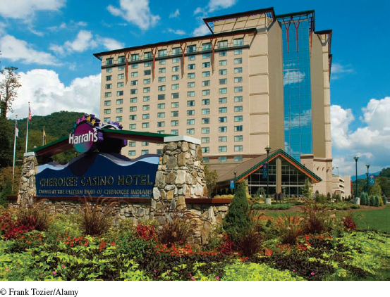
Revenue Management at Harrah's
Revenue management is a common practice in hotels, restaurants, and airlines, but nobody does it better than Harrah's Cherokee Casino and Hotel.
Consider this scenario. On a typical Thursday evening at the Cherokee, 183 of its 576 rooms are still unreserved for tomorrow night.
Customer: "I'd like to reserve a room for tomorrow night."
Operator: "May I have your Total Rewards number?"
Customer: "108578902."
Operator: "I'm sorry, Mr. Smith, all the rooms at the Cherokee are booked. Would you like me to make you a reservation at the Ramada? The room will be complimentary, of course."
Turning away a customer when there are vacancies and then giving the customer a free room at another hotel may seem crazy, but that's how Harrah's revenue management system works. From past data on customer expenditures, including gambling at the casinos, the hotel can calculate the "payoff" of each customer. Combined with statistical forecasts of demand by day of the week, time of the year, and under certain weather and other conditions, Harrah can determine whether it is likely that other customers (who are more profitable) will arrive and occupy those remaining rooms.
Granted, casinos are a special case, but the rewards of revenue management can be lucrative, an additional 15% in customer money spent at Harrah's. Going to a casino may be an "impulse" buy, but the impulse can be accurately predicted based on past behavior, given the right data. That's where the Total Rewards card comes in. Customers don't mind using the card for purchases or bets because it earns them free dinners, games, and other benefits. The quantitative model that decides whether to book a customer or not uses an exponential smoothing forecasting model, linear programming, and traditional marginal analysis (which we call revenue management).
Does the concept of revenue management surprise you? Can you think of a time when you have paid a different price because of your customer "class"?
Would there be times when it would not be appropriate (even illegal) to segment customers and give some customers special deals?
How do you think customers would respond if they knew about these practices?
Source: Richard Metters, Carrie Queenan, Mark Ferguson, et. al., "The 'Killer Application' of Revenue Management: Harrah's Cherokee Casino & Hotel," Interfaces, 38 (3), p. 161–175.
The useful life for products such as newspapers, flowers, baked goods, and seasonal items is so short that in many instances only one order for production can take place. Determining the size of that single order can be difficult.
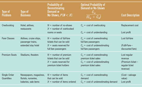
Table 14.4 shows the various types of revenue management problems with cost descriptions. In each of these problems, the cost of overestimating demand (times the probability that it will occur) must be balanced with the cost of underestimating demand and its probability of occurrence.
The optimum probability is where the cost of underestimating demand is equal to or just greater than the cost of overestimating demand. The derivation of the formula is shown below, followed by an example.
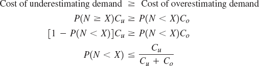
where
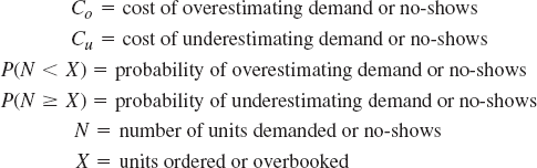
Given cost information and a distribution of demand or no-shows from past data, we can now match our planning policy with the optimum probability of overestimating demand. Example 14.6 illustrates the procedure for overbooking. A single order quantity problem is included in the solved problems at the end of this chapter.
Types of Revenue Management Problems
Lauren Lacy, manager of the Lucky Traveler Inn in Las Vegas, is tired of customers who make reservations and then don't show up. Rooms rent for $100 a night and cost $25 to maintain per day. Overflow customers can be sent to the Motel 7 for $70 a night. Lauren's records of no-shows over the past six months are given below. Should the Lucky Traveler start overbooking? If so, how many rooms should be overbooked?
No-Shows | Probability |
|---|---|
0 | 0.15 |
1 | 0.25 |
2 | 0.30 |
3 | 0.30 |
Solution
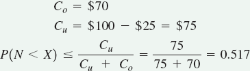
Adding a cumulative probability column of no-shows being less than expected gives us:
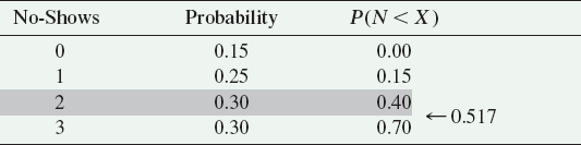
The optimal probability of no-shows falls between 0.40 and 0.70. Since we are concerned with no-shows less than or equal to 0.517 we choose the next lowest value, or 0.40. Following across the table, the Lucky Traveler should overbook by two rooms.
Sales and Operations Planning (S&OP) is a structured collaborative process for matching supply and demand. The sales plan and operations plan are expressed in aggregate terms, hence the name aggregate planning.
Aggregate planning is critical for companies with seasonal demand patterns and for services. Variations in demand can be met by adjusting capacity or managing demand. There are several mathematical techniques for aggregate planning, including linear programming, linear decision rule, search decision rule, and management coefficient model.
Production and capacity plans are developed at several levels of detail. The process of deriving more detailed production and capacity plans from the aggregate plan is called disaggregation. Collaborative planning sets production plans in concert with suppliers and trading partners. Available-to-promise often involves collaboration along a supply chain.
Aggregate planning for services is somewhat different from that for manufacturing because the variation in demand is usually more severe and occurs over shorter time frames. Fortunately, the constraining resource in most services is labor, which is quite flexible. Services use part-time workers, overtime, and undertime. Revenue management is a special aggregate planning tool for industries with time-sensitive products and segmented customer classes.
aggregate planning the process of determining the quantity and timing of production over an intermediate time frame.
available-to-promise the quantity of items that can be promised to the customer; the difference between planned production and customer orders already received.
backlog accumulated customer orders to be completed at a later date.
backordering ordering an item that is temporarily out-of-stock.
capable-to-promise the quantity of items that can be produced and made available at a later date.
chase demand an aggregate planning strategy that schedules production to match demand and absorbs variations in demand by adjusting the size of the workforce.
collaborative planning sharing information and synchronizing production plans across the supply chain.
disaggregation the process of breaking down the aggregate plan into more detailed plans.
level production an aggregate planning strategy that produces units at a constant rate and uses inventory to absorb variations in demand.
linear decision rule (LDR) a mathematical technique for aggregate planning.
lost sales forfeited sales for out-of-stock items
management coefficients model A regression technique for aggregate planning.
mixed strategy varying two or more capacity factors to determine a feasible production plan.
peak demand staffing for high levels of customer service.
pure strategy varying only one capacity factor in aggregate planning.
sales & operations planning (S&OP) a process for coordinating supply and demand
search decision rule (SDR) a pattern search technique for aggregate planning.
revenue management the process of determining the percentage of seats or rooms to be allocated to different fare classes.
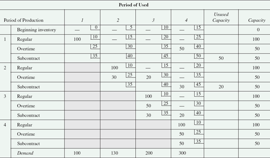
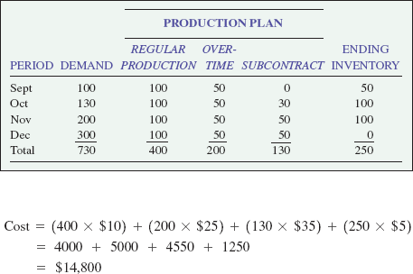
Fabulous Fit Fibers produces a line of sweatclothes that ex-hibits a varying demand pattern. Given the following demand forecasts, production costs, and constraints, design a production plan for Fabulous Fit using the transportation method of LP. Also, calculate the cost of the production plan.
PERIOD
DEMAND
September
100
October
130
November
200
December
300
Maximum regular production
100 units/month
Maximum overtime production
50 units/month
Maximum subcontracting
50 units/month
Regular production costs
$10/unit
Overtime production costs
$25/unit
Subcontracting costs
$35/unit
Inventory holding costs
$5/unit/month
Beginning inventory
0
SOLUTION
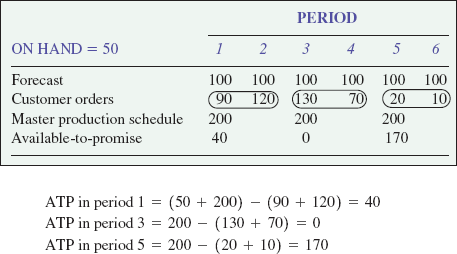
Calculate the available-to-promise for periods 1, 3, and 5.
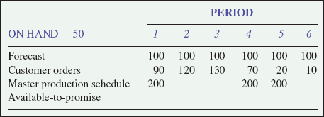
SOLUTION
Doughman Bakery bakes a variety of pastries, but none is more popular than its jumbo doughnuts. Doughnuts are made fresh every morning at 4:00 a.m. and sold throughout the day. Leftover doughnuts are put in a grab bag and sold at 75% discount the next day. Fresh doughnuts are sold for $1.20 each. The cost to make each doughnut is $0.45. The bakery has recorded first-day sales data for the last 200 days. Determine how many doughnuts Doughman Bakery should bake in the morning.
DOZENS OF DOUGHNUTS
FREQUENCY
2
14
3
18
4
26
5
32
6
30
7
26
8
20
9
18
10
12
11
2
12
2
SOLUTION
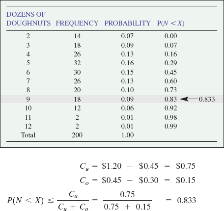
Doughman should make 9 dozen doughnuts.
14-1. What is the purpose of sales and operations planning? Describe the S&OP Process.
14-2. List several alternatives for adjusting capacity. List several alternatives for managing demand.
14-3. Describe the output of aggregate planning. When is aggregate planning most useful?
14-4. How do linear programming, the linear decision rule, the search decision rule, and the management coefficients model differ in terms of cost functions and output?
14-5. Identify several industries that have highly variable demand patterns. Explore how they adjust capacity.
14-6. What options are available for altering the capacity of (a) an elementary school, (b) a prison, and (c) an airline?
14-7. Discuss the advantages and disadvantages of using parttime workers, subcontracting work, and building up inventory as strategies for meeting demand.
14-8. Describe the levels of production and capacity planning in the hierarchical planning process.
14-9. Explain the process of collaborative planning. How is available-to-promise involved?
14-10. Access a major vendor of business software, such as SAP or Oracle. Read about their demand management, available-to-promise, and production planning products. What kinds of capabilities do these systems have?
14-11. How is the aggregate planning process different when used for services rather than for manufacturing?
14-12. What does revenue management entail? What types of businesses, besides hotels and airlines, would benefit from revenue management? As a consumer, how do you view the practice?
14-1. Bioway, Inc., a manufacturer of medical supplies, uses aggregate planning to set labor and inventory levels for the year. While a variety of items are produced, a standard kit composed of basic supplies is used for planning purposes. Demand varies with seasonal illnesses and the quarterly ordering policies of hospitals. The average worker at Bioway can produce 1000 kits a month at a cost of $9 per kit during regular production hours and $10 a kit during overtime production. Completed kits can also be purchased from outside suppliers at $12 each. Inventory carrying costs are $2 per kit per month. Overtime is limited to regular production, but subcontracting is unlimited. Due to high quality standards and extensive training, hiring and firing costs are $1500 per worker. Bioway currently employs 25 workers. Given the demand forecast below, develop a sixmonth aggregate production plan for Bioway using (a) chase demand and (b) a mixed strategy where the current workforce is kept for April through August, and supplemented with overtime and subcontracting as needed.
Month | Demand |
|---|---|
April | 60,000 |
May | 22,000 |
June | 15,000 |
July | 46,000 |
August | 80,000 |
September | 15,000 |
14-2. Demand for Quiggly Pops follows an up and down pattern over the four quarters of a year, with peaks in the spring and winter months when special promotions are held. Production is handled by a highly skilled local workforce during a regular 40-hour week (i.e., overtime and subcontracting are not used). The company likes to zero out its inventory at the end of a year so that it can start fresh each January. QP currently uses a level production strategy but would like to evaluate other options. Create a production plan and calculate the cost of the plan for each strategy listed below. Which plan would you recommend to QP?
Level production
Chase demand
Produce 70,000 in period 1, and 100,000 in periods 2 through 4.
Produce 90,000 in periods 1 through 3, and 100,000 in period 4.
Beginning workforce = 40 workers
Production per employee = 1,250 units per quarter
Quarter | Demand Forecast |
|---|---|
1 | 70,000 |
2 | 100,000 |
3 | 50,000 |
4 | 150,000 |
Hiring cost = $500 per worker
Firing cost = $500 per worker
Inventory carrying cost = $1 per unit per quarter
Regular production cost = $10 per unit
14-3. Rowley Apparel, manufacturer of the famous "Race-A-Rama" swimwear line, needs help planning production for next year. Demand for swimwear follows a seasonal pattern, as shown here. Given the following costs and demand forecasts, test these four strategies for meeting demand: (a) level production with overtime and subcontracting, as needed, (b) level production with backorders as needed, (c) chase demand, and (d) 3000 units regular production from April through September and as much regular, overtime, and subcontracting production in the other months as needed to meet annual demand. Determine the cost of each strategy. Which strategy would you recommend?
Month | Demand Forecast |
|---|---|
January | 1000 |
February | 500 |
March | 500 |
April | 2000 |
May | 3000 |
June | 4000 |
July | 5000 |
August | 3000 |
September | 1000 |
October | 500 |
November | 500 |
December | 3000 |
Beginning workforce | 8 workers |
Subcontracting capacity | unlimited |
Overtime capacity | 2000 units/month |
Production rate per worker | 250 units/month |
Regular wage rate | $15 per unit |
Overtime wage rate | $25 per unit |
Subcontracting cost | $30 per unit |
Hiring cost | $100 per worker |
Firing cost | $200 per worker |
Holding cost | $0.50 per unit/month |
Backordering cost | $10 per unit/month |
14-4. Mama's Stuffin' is a popular food item during the fall and winter months, but it is marginal in the spring and summer. Use the following demand forecasts and costs to determine which of the following production planning strategies is best for Mama's Stuffin':
Level production over the 12 months.
Produce to meet demand each month. Absorb variations in demand by changing the size of the workforce.
Keep the workforce at its current level. Supplement with overtime and subcontracting as necessary.
Month | Demand Forecast |
|---|---|
March | 2000 |
April | 1000 |
May | 1000 |
June | 1000 |
July | 1000 |
August | 1500 |
September | 2500 |
October | 3000 |
November | 9000 |
December | 7000 |
January | 4000 |
February | 3000 |
Overtime capacity per month | regular production |
Subcontracting capacity per month | unlimited |
Regular production cost | $30 per pallet |
Overtime production cost | $40 per pallet |
Subcontracting cost | $50 per pallet |
Holding cost | $2 per pallet |
Beginning workforce | 10 workers |
Production rate | 200 pallets per worker per month |
Hiring cost | $5000 per worker |
Firing cost | $8000 per worker |
14-5. FansForYou is a small, privately owned company that manufactures fans. Large variations in demand due to seasonality have contributed to high costs for the company. FansForYou currently uses a level production strategy because it prefers not to hire and fire employees. However, if there is enough cost justification, the company will consider alternative production plans.
What is the cost of the current production plan?
How much would FansForYou save by using a chase demand strategy?
How much would FansForYou save by keeping a steady workforce of 20 workers and supplementing with overtime and subcontracting as needed?
Month | Demand |
|---|---|
September | 1500 |
October | 1000 |
November | 600 |
December | 600 |
January | 600 |
February | 800 |
March | 1000 |
April | 1000 |
May | 4000 |
June | 6500 |
July | 6000 |
August | 4000 |
Beginning inventory | 0 |
Beginning workforce | 25 workers |
Production rate | 100 fans per worker per month |
Regular production cost | $40 per fan |
Overtime production cost | $60 per fan |
Subcontracting cost | $70 per fan |
Overtime capacity | Not to exceed regular production |
Subcontracting capacity | Unlimited |
Holding cost | $8 per fan |
Hiring cost | $2000 |
Firing cost | $3000 |
14-6. Slopes & Sleds (S&S) makes skis, snowboards, and highend sledding equipment. As shown below, the demand for its products is highly seasonal. The company employs 10 workers who can each produce 200 units of various equipment per month. The cost of regular production is $8 per unit, overtime $12, and subcontracting $16. Overtime is limited to regular production each period. Subcontracting is unlimited. Hiring and firing costs are $500 per worker. Inventory holding costs are $2 per unit per month. Given the estimates of demand below, create an aggregate production plan for Slopes & Sleds using:
the current workforce level (supplemented with overtime and subcontracting as needed),
chase demand.
Month | Demand |
|---|---|
January | 6400 |
February | 7000 |
March | 1500 |
April | 500 |
May | 600 |
June | 1400 |
July | 1600 |
August | 2000 |
September | 1400 |
October | 1500 |
November | 5200 |
December | 6900 |
14-7. Sawyer Furniture is one of the few remaining domestic manufacturers of wood furniture. In the current competitive environment, cost containment is the key to its continued survival. Demand for furniture follows a seasonal demand pattern with increased sales in the summer and fall months, culminating with peak demand in November.
The cost of production is $16 per unit for regular production, $24 for overtime, and $33 for subcontracting. Hiring and firing costs are $500 per worker. Inventory holding costs are $20 per unit per month. There is no beginning inventory. Ten workers are currently employed. Each worker can produce 50 pieces of furniture per month. Overtime cannot exceed regular production. Given the following demand data, design an aggregate production plan for Sawyer Furniture that will meet demand at the lowest possible cost.
In an attempt to stem the flow of jobs overseas, the local labor union has negotiated a penalty clause for layoffs. The new contract increases the firing cost per worker to $2500. Create a revised aggregate plan with these new cost figures. Assuming any subcontracting is, in fact, foreign production, does the penalty work? Why or why not?
Month | Demand |
|---|---|
January | 500 |
February | 500 |
March | 1000 |
April | 1200 |
May | 2000 |
June | 400 |
July | 400 |
August | 1000 |
September | 1000 |
October | 1500 |
November | 7000 |
December | 500 |
14-8. Midlife Shoes, Inc. is a manufacturer of sensible shoes for aging baby-boomers. The company is having great success, and although demand is seasonal, it is expected to increase steadily over the next few years. The company is purchasing a new facility to accommodate the increase in demand, but the facility will not open until 13 months from now. The current facility can only accommodate 15 workers. Hiring and firing costs are negligible. Using the information below, help Midlife manage this transition year by deriving a production plan that will meet demand at the lowest cost. With the limited workforce size, neither chase demand nor level production is viable.
Month | Demand |
|---|---|
January | 1000 |
February | 1200 |
March | 1200 |
April | 3000 |
Month | Demand |
|---|---|
May | 3000 |
June | 3000 |
July | 2200 |
August | 2200 |
September | 4000 |
October | 4000 |
November | 2200 |
December | 3000 |
Beginning inventory | 0 units |
Beginning workforce | 8 workers |
Production rate | 100 units per worker per month |
Regular capacity | Maximum of 15 workers |
Overtime capacity | Half of regular production |
Subcontracting capacity | 1000 units |
Regular production cost | $36 per unit |
Overtime production cost | $54 per unit |
Subcontracting cost | $70 per unit |
Inventory holding cost | $10 per unit |
14-9. Design a production plan for Rowley Apparel in Problem 14-3 using linear programming and Excel Solver.
14-10. Design a production plan for Mama's Stuffin' in Problem 14-4 using linear programming and Excel Solver.
14-11. Design a production plan for FansForYou in Problem 14-5 using linear programming and Excel Solver.
14-12. Design a production plan for Slopes and Sleds in Problem 14-6 using linear programming and Excel Solver.
14-13. The global sourcing department of Slopes and Sleds (see Problems 14-6 and 14-12) has located a company in China that can make S&S products for $9 a unit. Revise the production plan using Solver. How much money can be saved by outsourcing to China? What other factors should be considered in the outsourcing decision?
14-14. The Wetski Water Ski Company is the world's largest producer of water skis. As you might suspect, water skis exhibit a highly seasonal demand pattern, with peaks during the summer months and valleys during the winter months. Given the following costs and quarterly sales forecasts, use the transportation method to design a production plan that will economically meet demand. What is the cost of the plan?
Quarter | Sales Forecast |
|---|---|
1 | 50,000 |
2 | 150,000 |
3 | 200,000 |
4 | 52,000 |
Inventory carrying cost | $3.00 per pair of skis per quarter |
Production per employee | 1000 pairs of skis per quarter |
Regular workforce | 50 workers |
Overtime capacity | 50,000 pairs of skis |
Subcontracting capacity | 40,000 pairs of skis |
Cost of regular production | $50 per pair of skis |
Cost of overtime production | $75 per pair of skis |
Cost of subcontracting | $85 per pair of skis |
14-15. College Press publishes textbooks for the college market. The demand for college textbooks is high during the beginning of each semester and then tapers off during the semester. The unavailability of books can cause a professor to switch adoptions, but the cost of storing books and their rapid obsolescence must also be considered. Given the demand and cost factors shown here, use the transportation method to design an aggregate production plan for College Press that will economically meet demand. What is the cost of the production plan?
Months | Demand Forecast |
|---|---|
February–April | 5,000 |
May–July | 10,000 |
August–October | 30,000 |
November–January | 25,000 |
Regular capacity per quarter | 10,000 books |
Overtime capacity per quarter | 5,000 books |
Subcontracting capacity per qtr | 10,000 books |
Regular production rate | $20 per book |
Overtime wage rate | $30 per book |
Subcontracting cost | $35 per book |
Holding cost | $2.00 per book |
14-16. Bits and Pieces uses overtime, inventory, and subcontracting to absorb fluctuations in demand. An annual production plan is devised and updated quarterly. Expected demand over the next four quarters is 600, 800, 1600, and 1900 units, respectively. The capacity for regular production is 1000 units per quarter with an overtime capacity of 100 units a quarter. Subcontracting is limited to 500 units a quarter. Regular production costs $20 per unit, overtime $25 per unit, and subcontracting $30 per unit. Inventory holding costs are assessed at $3 per unit per period. There is no beginning inventory. Design a production plan that will satisfy demand at minimum cost.
14-17. GF Incorporated, a manufacturer of power systems, uses overtime, inventory, and subcontracting to absorb fluctuations in demand. An annual production plan is devised and updated quarterly. The expected demand and available capacities for the next four quarters are as follows:
Period | Demand | Regular Capacity | Overtime Capacity | Subcontracting Capacity |
|---|---|---|---|---|
1 | 2000 | 1000 | 1000 | 5000 |
2 | 4500 | 1000 | 1000 | 5000 |
3 | 7500 | 1000 | 1000 | 5000 |
4 | 3000 | 1000 | 1000 | 5000 |
Relevant cost data are as follows:
Regular production cost per unit | $20 |
Overtime production cost per unit | $25 |
Subcontracting cost per unit | $30 |
Inventory holding cost per unit per period | $ 3 |
Beginning inventory | 0 |
Design a production plan that will satisfy demand at minimum cost.
14-18. Caltex uses overtime, inventory, and subcontracting to absorb fluctuations in demand. An annual production plan is devised and updated quarterly. Expected demand, available capacities, and costs for the next four quarters are given below. Design a production plan that will satisfy demand at minimum cost.
Period | Demand | Regular Capacity | Overtime Capacity | Subcontracting Capacity |
|---|---|---|---|---|
1 | 1500 | 1000 | 200 | 500 |
2 | 1900 | 1000 | 200 | 500 |
3 | 500 | 1000 | 200 | 500 |
4 | 2000 | 1000 | 200 | 500 |
Regular production cost per unit | $10 |
Overtime production cost per unit | $15 |
Subcontracting cost per unit | $20 |
Inventory holding cost per unit per period | $ 2 |
14-19. MTI, a global telecommunications company, manufactures cable boxes and DVRs for its customers. Demand varies considerably from quarter to quarter. Using the demand, capacities, and cost figures given below, devise an aggregate production plan for MTI that minimizes costs.
Period | Demand | Regular Capacity | Overtime Capacity | Subcontracting Capacity |
|---|---|---|---|---|
1 | 500 | 1000 | 200 | 500 |
2 | 1200 | 1000 | 200 | 500 |
3 | 2500 | 1000 | 200 | 500 |
4 | 1900 | 1000 | 200 | 500 |
Regular production cost per unit | $20 |
Overtime production cost per unit | $25 |
Subcontracting cost per unit | $30 |
Inventory holding cost per unit per period | $ 3 |
14-20. Robotic Pet Products uses overtime, inventory, and subcontracting to absorb fluctuations in demand. As expected, demand in the fourth quarter during the holiday season is particularly high, followed by first quarter demand for customers purchasing accessories for their Rpets. Given the demand and available capacities shown below, design a production plan that will satisfy demand at minimum cost.
Period | Demand | Regular Capacity | Overtime Capacity | Subcontracting Capacity |
|---|---|---|---|---|
1 | 1000 | 1000 | 100 | 500 |
2 | 800 | 1000 | 100 | 500 |
3 | 600 | 1000 | 100 | 500 |
4 | 2600 | 1000 | 100 | 500 |
Regular production cost per unit | $10 |
Overtime production cost per unit | $15 |
Subcontracting cost per unit | $20 |
Inventory holding cost per unit per period | $3 |
Beginning inventory | 100 |
14-21. How many units are available-to-promise in period 1? period 4?
On hand = 60 | Period | |||||
|---|---|---|---|---|---|---|
1 | 2 | 3 | 4 | 5 | 6 | |
Forecast | 50 | 100 | 100 | 100 | 100 | 50 |
Customer Orders | 85 | 125 | 95 | 85 | 45 | 15 |
Master Production Schedule | 250 | 250 | ||||
Available-to-Promise | ||||||
14-22. Complete the available-to-promise table below.
On hand = 10 | Period | |||||
|---|---|---|---|---|---|---|
1 | 2 | 3 | 4 | 5 | 6 | |
Forecast | 50 | 50 | 50 | 50 | 50 | 50 |
Customer Orders | 56 | 17 | 75 | 50 | 16 | 14 |
Master Production Schedule | 100 | 100 | 100 | |||
Available-to-Promise | ||||||
14-23. Complete the available-to-promise table below.
On hand = 30 | Period | |||||
|---|---|---|---|---|---|---|
1 | 2 | 3 | 4 | 5 | 6 | |
Forecast | 100 | 50 | 100 | 50 | 100 | 50 |
Customer Orders | 75 | 50 | 116 | 73 | 45 | 23 |
Master Production Schedule | 100 | 50 | 100 | 50 | 100 | 50 |
Available-to-Promise | ||||||
14-24. Calculate the available-to-promise row in the following matrix.
On hand = 100 | Period | |||||
|---|---|---|---|---|---|---|
1 | 2 | 3 | 4 | 5 | 6 | |
Forecast | 50 | 100 | 50 | 100 | 50 | 100 |
Customer Orders | 50 | 125 | 75 | 175 | 45 | 15 |
Master Production Schedule | 200 | 200 | ||||
Available-to-Promise | ||||||
14-25. How many B's are available-to-promise in week 2? How soon could you fill an order for 250 B's?
On hand = 10 | Period | |||||
|---|---|---|---|---|---|---|
1 | 2 | 3 | 4 | 5 | 6 | |
Forecast | 100 | 100 | 100 | 100 | 100 | 100 |
Customer orders | 25 | 50 | 137 | 72 | 23 | 5 |
Master production schedule | 100 | 100 | 100 | 100 | 100 | 100 |
Available-to-Promise | ||||||
14-26. Managers at the Dew Drop Inn are concerned about the increasing number of guests who make reservations but fail to show up. They have decided to institute a policy of overbooking like larger hotel chains. The profit from a paying guest averages $50 per room per night. The cost of putting up a guest at another hotel is $100 per room per night. Records show the following number of no-shows over the past three months:
No-Shows | Frequency |
|---|---|
0 | 18 |
1 | 36 |
2 | 27 |
3 | 9 |
How many rooms should Dew Drop overbook?
14-27. Atlanta Airlines routinely overbooks its flight from Atlanta to Boston. Overbooking discounted seats can be expensive because providing a bumped passenger with a last-minute flight on a competing carrier can cost $450. A 120-passenger jet costs about $6000 to operate from Atlanta to Boston. The average ticket price is $300.
Given the frequency of no-shows in the following table, how many seats should be overbooked?
Atlanta Air offers special rates on its Atlanta/Boston route for the holidays. How would a $200 ticket price affect the number of seats overbooked?
No-Shows | Frequency |
|---|---|
1 | 15 |
2 | 10 |
3 | 10 |
4 | 5 |
5 | 3 |
6 | 5 |
14-28. The Blue Roof Inn overbooks two rooms a night. Room rates run $100 a night but cost only $30 to maintain. Bumped customers are sent to a nearby hotel for $80 a night. What is the cost of overbooking? What is the cost of underbooking? Given the following distribution of no-shows, should Blue Roof continue its current policy?
No-Shows | Probability |
|---|---|
0 | 0.30 |
1 | 0.20 |
2 | 0.10 |
3 | 0.30 |
4 | 0.10 |
14-29. FlyUs Airlines is unhappy with the number of empty seats on its New York to Philadelphia flight. To remedy the problem, the airline is offering a special discounted rate of $89 instead of the normal $169, but only for 7-day advance purchases and for a limited number of seats per flight. The aircraft flown from NY to Philly holds 100 passengers. Last month's distribution of full-fare passengers is shown below. How many seats should FlyUs reserve for full-fare passengers?
Full-Fare | Frequency |
|---|---|
50 | 15 |
55 | 20 |
60 | 35 |
65 | 20 |
70 | 10 |
14-30. NorthStar Airlines runs daily commuter flights from Washington, D.C., to Chicago. The planes hold 60 passengers and cater to the business traveler with comparable business rates. The recent economic downturn has reduced the occupancy rate of flights to such an extent that NorthStar would like to offer a set number of seats at discount rates to gain more passengers. The board of directors is worried that discounted seats will cut into profit margins and will upset the regular business traveler. The ticket price for a business traveler is $350. Discounted tickets would sell for $120. Assuming that empty seats can be sold if discounted, use the following data gathered from 100 flights to determine how many seats should be discounted.
No. of Full-Fare Passengers | Frequency |
|---|---|
10 | 15 |
20 | 25 |
30 | 25 |
40 | 20 |
50 | 10 |
60 | 5 |
14-31. The Forestry Club sells Christmas trees each year to raise money for club activities. The trees cost $10 to cut and are sold for $25. Unused trees are stripped of their limbs and sold as firewood for $1 apiece. Data on past sales appear below. How many trees should the forestry club cut this year?
No. of Full-Fare Passengers | Frequency |
|---|---|
10 | 6 |
15 | 3 |
20 | 6 |
25 | 3 |
30 | 2 |
14-32. Pizza Pie runs the pizza concessions at the University basketball games. Personal size pizzas are assembled two hours prior to the game and cooked throughout the night in a mobile oven outside of the coliseum. Pizza sells for $5 and costs approximately $2 to make. Unsold pizzas at the end of the game are given to nearby dormitory students for a nominal $1 per pizza. Having sold out of pizza during the past two games, Pizza Pie is reevaluating its planning policy. Use the past demand data given below to determine how many pizzas should be made for each game.
No. of Full-Fare Passengers | Frequency |
|---|---|
25 | 15 |
50 | 15 |
75 | 30 |
100 | 20 |
125 | 10 |
150 | 10 |
14-33. Tariott Hotel rents rooms for $125 a night that cost approximately $50 per day to maintain. Overbooking is a common practice in the industry. Customers whose rooms have been leased to someone else are put up in a nearby hotel for $100 a night. Records show that during the past month, there were 10 days with zero no-shows, 5 days with 1 no-show, 6 days with 2 no-shows, and 9 days with 3 no-shows.
What is the cost of overbooking?
What is the cost of underbooking?
What is the optimum probability of no-shows for Tariott?
How many rooms should Tariott overbook?
Seats for Sale
Blokie State's football program has risen to the ranks of the elite with postseason bowl games in each of the past 10 years, including a national championship game. The Blokes (as the fans are called) fill the stadium each game. Season tickets are increasingly difficult to find. In response to the outstanding fan support, Blokie State has decided to use its bowl revenues to expand the stadium to 75,000 seats.
The administration is confident that all 75,000 seats can be sold at the normal price of $40 per game ticket; however, Frank Pinto's job, as athletic director, is to get as much revenue out of the stadium expansion as possible. In addition to stadium boxes for the truly endowed, Frank would like to take this opportunity to repurpose existing seats. A certain number of seats (yet to be determined) would be set aside for premium ticket holders who would pay $200 per ticket for the privilege of 50-yard line seats with chair backs and access to indoor concessions. The question is, how many fans would be willing to pay such a premium? If too many seats are designated in the premium sections, they could remain vacant. Too few premium seats would lose potential revenue for the program.
Frank has decided that if the plan has any chance of success, unsold premium seats should not be sold at reduced rates. It would be better to donate them to local charities instead. Gathering data from his cohorts at peer institutions, Frank has put together the following probability distribution of premium ticket holders. The data begin with 1000 tickets since Frank already has requests for 999 tickets from alumni donors. He is asking for your help in performing the analysis.
No. of Premium Tickets | Probability |
|---|---|
1,000 | 0.10 |
5,000 | 0.30 |
10,000 | 0.24 |
15,000 | 0.15 |
20,000 | 0.10 |
25,000 | 0.06 |
30,000 | 0.05 |
Using revenue management, determine how many seats should be reserved for premium ticket holders.
Considering your answer to part (a) and the possible outcomes listed above, how much total revenue (i.e., regular and premium) can be expected from ticket sales?
The administration is unsure about Frank's plan. The VP of Finance thinks an expected value of the number of premium seats would produce better results. How would the number of premium seats change using expected value? Considering the possible outcomes, which approach yields the most potential revenue? (See Supplement 1 for an explanation of expected value.)
Erin's Energy Plan
The discussion was getting heated. A brightly colored chart at the front of the room told the story all too well. At Waylan Industries sales were up, profits down.
"Larry, there's no way we can hit our profit objective with your high cost of production. You've got to cut back."
"Why pick on me? We're running bare bones as it is. Last winter's energy prices really killed us. How can you cut costs with a 250% increase in energy prices?"
Everyone stared at Erin. Erin swallowed hard and spoke up. "You know, we've never had to stockpile fuel before and I'm not sure how far we can go in managing demand, but I've been collecting data on purchase options. . . . "
"Well, let's see it then."
"Although it's not how we purchase energy, I've converted the prices to millions of BTUs for comparison. Coal costs $8 per million BTUs, but we can only burn 500 million per quarter to stay within our environmental air standards. Natural gas costs $32 per million BTUs, and petroleum $46. We can burn 1000 million BTUs of each per quarter. Coal and natural gas can be stored for later use at a holding cost of 30 percent of purchase price per quarter. The holding cost for petroleum is 20 percent. Electricity cannot be stored, but it can be reserved in advance. The cost of electricity also varies considerably by season of the year, as do our energy needs. The cost of electricity from the local utility is $20 per million BTUs in the spring, $40 in the summer, $24 in the fall, and $70 in the winter. These are averages from last year. A nearby utility quotes slightly higher prices at $22, $44, $26, and $75 for spring, summer, fall, and winter. As far as availability is concerned, 4000 million BTUs of electricity are available in the spring and fall, 5000 in the summer and winter. We can save some money by contracting with the utilities in advance of the season. I've summarized the options in the table here, along with our energy needs. What I need now is some help analyzing the data. Larry, could you . . ."
Before Erin could finish, Tom spoke up. "Yes, Larry—you and Erin work up an energy plan—like those aggregate production plans you're always bringing in. And have it ready by Thursday."
Source: This case was developed with the help of Richard Hirsh, Professor of Science and Technology at Virginia Tech.
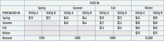
Use Erin's data to develop an aggregate energy plan for Waylan Industries.
Bowman, E. H. "Production Planning by the Transportation Method of Linear Programming." Journal of Operations Research Society (February 1956), pp. 100–103.
Bowman, E. H. "Consistency and Optimality in Managerial Decision Making." Management Science (January 1963), pp. 310– 321.
Buffa, E. S., and J. G. Miller. Production-Inventory Systems: Planning and Control, 3rd ed. Homewood, IL: Irwin, 1979.
Correll, J., and N. Edson. Gaining Control. New York: Wiley, 1998.
Haksever, C., B. Render, and R. Russell and R. Murdick. Service Operations and Management. Upper Saddle River, NJ: Prentice Hall, 2000.
Holt, C., F. Modigliani, J. Muth, and H. Simon. Planning Production, Inventories and Work Force. Englewood Cliffs, NJ: Prentice Hall, 1960.
Palmatier, G. E. and C. Crum. Enterprise Sales and Operations Planning. Boca Raton: J. Ross Publishers, 2003.
SAP AG. "Global Available to Promise." December 1999. SAP AG 2000, APO ATP 3.0. http://www.sap.com/solutions/scm/apo/pdf/atp.pdf.
Taubert, W. "A Search Decision Rule for the Aggregate Scheduling Problem." Management Science (February 1968), pp. B343–359.
Tersine, R. Production/Operations Management: Concepts, Structure, and Analysis. New York: Elsevier-North Holland, 1985.
Vollmann, T., W. Berry, and D. C. Whybark. Manufacturing Planning and Control Systems, 4th ed. Homewood, IL: Irwin, 1997.
Wallace, T. Sales and Operations Planning—The How-to Handbook. Columbus, OH: T. F. Wallace & Co., 2000.
[20] For this example, our initial solution to the production problem happens to be optimal. In other cases, it may be necessary to iterate to additional transportation tableaux before an optimal solution is reached. Students unfamiliar with the transportation method should review the topic in the Supplement to Chapter 10.