The first step is very straightforward. Here, we use the metacoder parse_qiime_biom() function to load in our biom file and then use subsetting on the resulting taxdata$data$otu_table slot to extract a simple OTU table into otu_table.

We can now call the diversity() function from vegan. The index argument is set to "simpson", so the function will use the Simpson index for within-sample diversity. The MARGIN argument tells the function whether the samples are in rows or columns: 1 for rows and 2 for columns. The diversity() function returns a named vector that is easy to visualize with the barplot() function, giving us this:

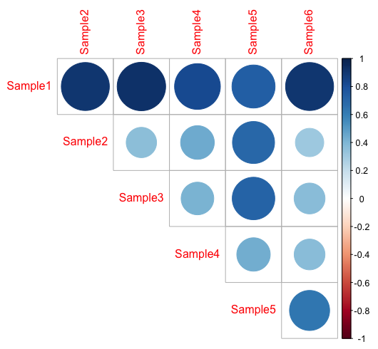
We can now run the between-sample diversity measure using the vegdist() function; again, the index argument sets the index to use, and here, we choose the Bray index. vegdist() expects the sample data to be rows, so we use the t() function to rotate otu_table. The resulting object is stored in between_sample— it's a pairwise correlation table and we can visualize it in corrplot. To do this, we need to convert it into a matrix with as.matrix(); the ncol argument should match the number of samples so that you get a column for each sample. The returned matrix, between_sample_m, can be passed to the corrplot() function to render it. By setting method to circle, type to upper, and diag to false, we get a plot with only the upper diagonal of the matrix, without the self-versus-self comparisons reducing redundancy in the plot.

The output looks like this: