In Step 1, we begin by reading in the arabidopsis.gff file, a file that describes the lengths of the chromosomes we'd like to use in our plot. We only needed the name, start, and end columns, so we piped the data to the dplyr::select() function to keep the appropriate columns, that is, X1, X4, and X5. As a .gff file has no column headings, the read_tsv() functions give the column names X1 ... Xn. We saved the result in the df object.

In Step 2, we started building the plot. We used the circos.genomicInitialize() function with df to create the plot's backbone and coordinate system and then manually added a single link. The circos.link() function allows us to create a single origin and destination using the chromosome's name, c(start, end) format, thereby coloring the link in the requested color. The plot currently looks like this:

At the start of Step 3, we used circos.clear() to completely reset the plot. Resetting is only necessary for the purposes of this tutorial as we want to build things step-wise; you can likely ignore it in your own coding. The next stage is to load in a file of genomic regions that represent the source of some links and a separate file of genomic regions that represent the target of some links. These two files should be in BED format and row N in the source file must correspond to row N in the target file. Then, we reinitialized the plot with circos.genomicInitialize() and used circos.genomicLink() to add many links in one command, passing it the objects of the source link data and the target data before coloring them all blue. The plot looks like this:

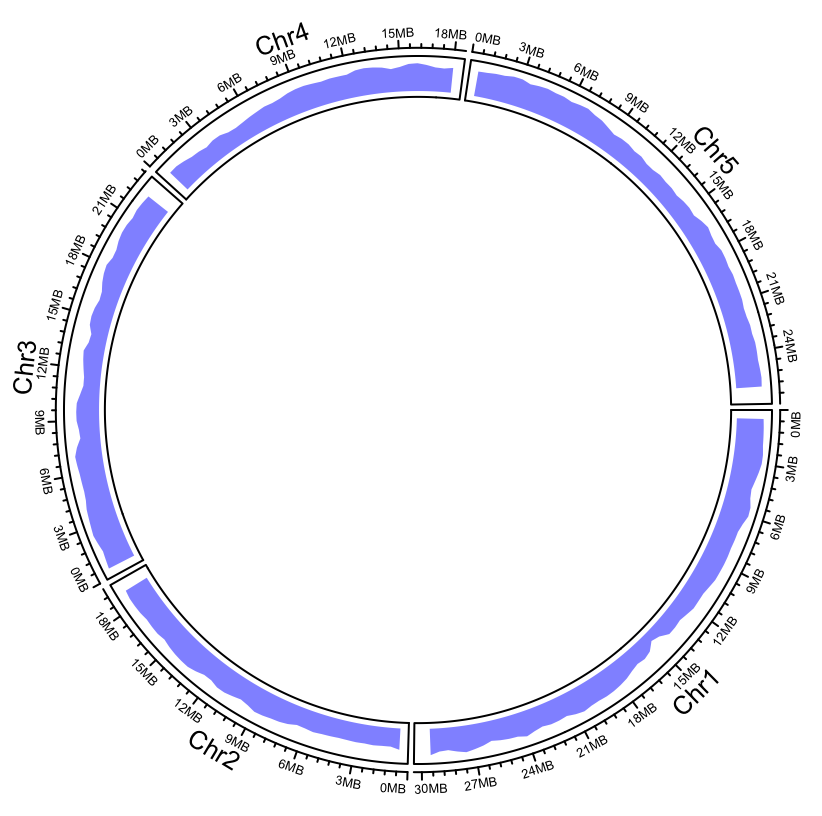
In Step 4, after clearing the plot, we read in another BED file of gene positions from arabidopsis_genes.bed. We want to add this information as a density track that counts the number of features in the windows of user-specified length and plots them as a density curve. To do this, we use the circos.genomicDensity() function, passing it the dataframe of gene_positions, selecting a window size of 1 million, a color (note the color is in the eight-digit HEX format that allows us to add transparency to the color), and track.height, which specifies the proportion of the plot to use for this track. The track looks like this:

In Step 5, we added a more complex track—a heatmap that can represent many columns of quantitative data. The file format here is extended BED format, with a chromosome name, start, and end with data in any further columns. We have three extra columns of data in our sample arabidopsis_quant_data.bed file. We load the bed file into heatmap_data with read.delim(). Next, we created a color function and saved it as col_fun to help draw the heatmap. The colorRamp2() function takes a vector of the minimum, middle, and maximum values of the data as its argument, for which the colors specified in the second argument should be used. So, with 10, 12, and 15 and green, red, and black, we drew 10 in green, 12 in black, and 15 in red, respectively. The colors for the values in-between those points are calculated automatically by colorRamp2(). To draw the heatmap, we used the circos.genomicHeatmap() function, passing col_fun to the col argument. The side argument specifies whether to draw inside or outside the circle, while the border argument specifies the color of the lines between heatmap elements. The plot looks like this:

Finally, in Step 6, we put all of this together. By clearing and reinitializing the plot, we specified the order of the tracks from outside to in by calling the relevant functions in outside first to inside last order:

The final plot, as seen in the preceding image, gets circos.genomicHeatmap(), then circos.genomicDensity(), and then circos.genomicLink() to give us the circular genome plot.