In the following example, we will load a dataset containing performance scores for employees. We will observe four records for each employee. For each time step, each employee will receive either the traditional or the boost compensation package. We want to find out whether there are differences between the two compensation packages:

1. First, we need to load the necessary libraries and the dataset that we will use: 

library(ggplot2)
library(nlme)
data_company = read.csv("./repeated_measures.csv")

2. We will plot the responses for each employee. Here, we want to determine whether the Time/Performance slopes are the same between employees or not. We can see that the slopes (Performance-Time) are similar, so it doesn't seem necessary to add a different time response for each employee:

ggplot(data_company,aes(x=Time,y=Performance)) + geom_line() +
geom_point(data=data_company,aes(x=Time,y=Performance)) +
facet_wrap(~Employee,nrow=3)

The preceding code generates the following output:

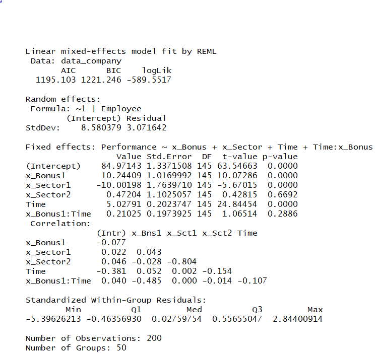
3. The fixed effects part will consist of the Bonus type, Sector (company department), Time, and a Time:Bonus type interaction. For the random effects part, we will only have a random intercept by Employee. We are also specifying an autoregressive order 1 (AR1) lag structure. This will cause every pair of consecutive observations for the same experimental unit to be correlated. The first thing we notice is the Akaike information criterion (AIC) number, which can be used to among different models. The random effects part contains the variance for the random effects, plus the variance for the residual. It can be seen that the Employee variance contributes 80% more variability than the residual. The Phi coefficient is the autoregressive coefficient for the residual. We then get the estimated coefficients for the fixed effects, along with the standard errors and the p-values:

fit <- lme(Performance ~ Bonus + Sector + Time + Time:Bonus , random = list( ~1 |Employee) , correlation = corAR1(form= ~Time|Employee), data = data_company)
 summary(fit)

The following screenshot shows the model results. We are testing whether there is an interaction between time and bonus. It is slightly non-significative, meaning that the impact of the bonus is independent of the time in the company:

4. The ANOVA table can be built using the following code. These F tests are consistent with what we have already seen in the fixed effects coefficients. All of the effects are significative, except for the TimexBonus interaction:

anova(fit)

The preceding code generates the following output for the anova table:

5. But do we really need the AR1 error term? The issue is that the more irrelevant terms we have in our model, the greater the imprecision will be for our main effects. So, we only want to keep the necessary parts of our model:

fit <- lme(Performance ~ Bonus + Sector + Time + Time:Bonus , random = list( ~1 |Employee) , data = data_company)
 summary(fit)
 anova(fit)

The following screenshot shows the simplified model with no autoregressive structure:

6. The AIC criterion can be used to choose the best model among a set of competing ones. The likelihood always increases with the more parameters we add because a more complex model always fits the data better. So, the likelihood itself cannot be used to determine which model should be used (it would just tell us to always use the more complex model). The AIC penalizes the log-likelihood by the number of parameters. Operationally, we just pick the model with the lowest AIC. As we can see, the model that does not include the AR1 coefficient has a lower AIC.
7. Consequently, we decide to use our starting model.
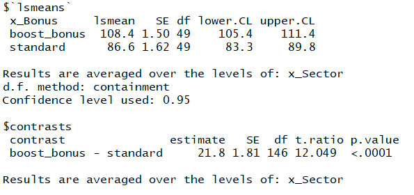
8. We finally calculate lsmeans. We can conclude that the boost_bonus pack provides a statistically significative increase in the performance score of 108.4 (note that, in this model formulation, we have removed the interaction). The contrast between boost_bonus and the standard bonus is highly significative as well, as we would expect:

library(lsmeans) 
fit <- lme(Performance ~ Bonus + Sector + Time , random = list( ~1 |Employee) , data = data_company) 
print(lsmeans(fit,pairwise ~ Bonus)) 

The preceding code generates the following output of the lsmeans results: