In the following example, we will load the house price dataset that we used in the previous recipe, and we will study how different priors impact the results:

1. We load the dataset and do our model. We will only put a prior on beta[6] in order to simplify our comparison. In the first case, we will put a flat prior—uniform (0,1000). We will only direct our attention toward the beta[6] posterior density; as we can see, the density is not very concentrated around 1:

data = read.csv("./house_prices.csv")
model ="
data {
real y[125];
real x[125,6];
}
parameters {
real beta[6];
real sigma;
real alpha;
}
model {
beta[1] ~ uniform(0,1000);
for (n in 1:125)
y[n] ~ normal(alpha + beta[1]*x[n,1] + beta[2]*x[n,2] + beta[3]*x[n,3] + beta[4]*x[n,4] + beta[5]*x[n,5] + beta[6]*x[n,6], sigma);
}"
xy = list(y=data[,1],x=data[,2:7])
fit = stan(model_code = model, data = xy, warmup = 500, iter = 1000, chains = 1, cores = 1, thin = 1,verbose=FALSE)
stan_dens(fit)

The following screenshot shows the posterior density: 

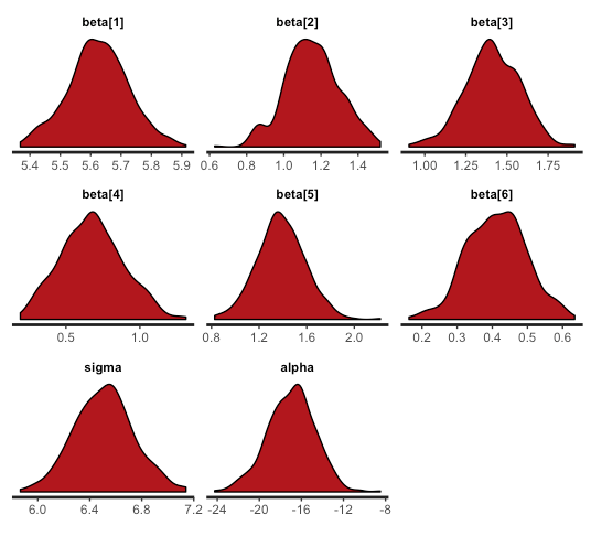
2. What would have happened if we had used different priors? We put very tight priors around one (priors so tight are seldom used). The posterior distributions are now almost centered around one (or much closer to one), as shown in the following code:

beta[1]  ~ uniform(0,1000);  
beta[2]  ~ normal(1,0.1);  
beta[3]  ~ normal(1,0.1);  
beta[4]  ~ normal(1,0.1);  
beta[5]  ~ normal(1,0.1);  
beta[6]  ~ normal(1,0.1);