In this recipe, we will use the sjPlot package to generate tables for lm and lmer outputs, and we will explore some of its basic capabilities:

1. Let's start by creating a table for a linear model estimated via lm. The tab_model function creates the output that we need based on a fitted model:

library(sjPlot) 
clients <- read.csv("./clients.csv") 
model1 <- lm(Sales ~ Strategy + (Client) + (Salesman),data=clients) tab_model(model1) 

The following screenshot shows the estimated coefficients (the <0.001 are highly significative):

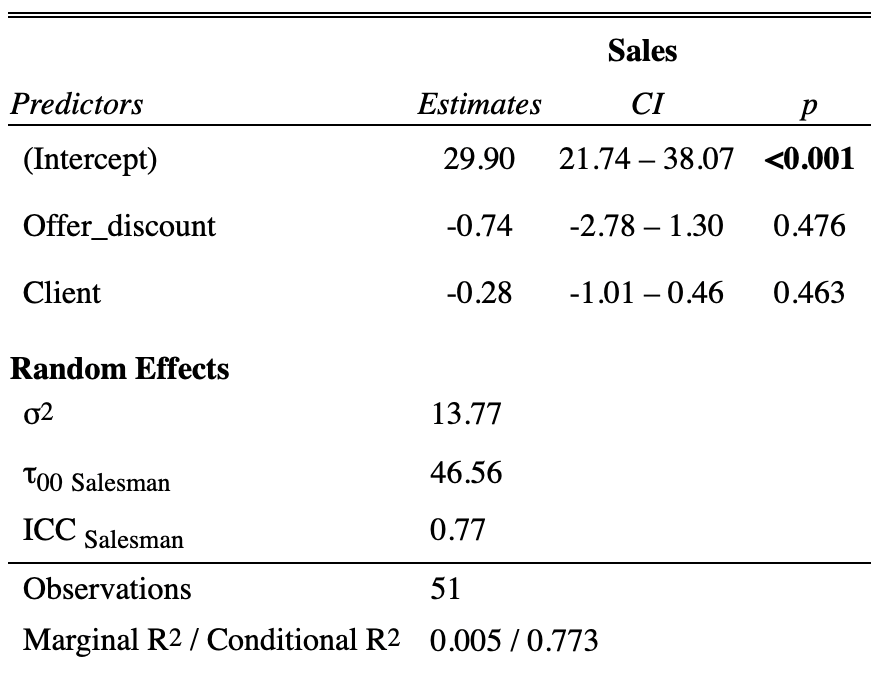
2. The tab_model function can be used with mixed effects models (the ones that include both fixed and random effects). Random effects are used when we want to model an effect as originating from a large (and possibly infinite) sample. For each random effect, we get a variance component, instead of getting one coefficient for each factor level in the effect (this is what happens for fixed effects):

model2 <- lmer(Sales ~ Strategy + (1|Client) + (1|Salesman),data=clients) 
tab_model(model2) 

The following screenshot shows the estimated coefficients for a mixed model: