In this exercise we will detect variables that are correlated using a dataset containing prices for several apparel categories. The target variable will be the sales, but we will need to make sure that we treat all the correlations accordingly.We will first load our dataset. It contains the following variables:

"Sales", "women_apparel_price", "male_apparel_price", "shoes_female_price", "shoes_male_price", "shoes_kids_prices", "shoes_male_price.1" and "prices_shoes".  

What we want to model are Sales in terms of all the other variables: female/male apparel price, female/male shoes price, female/kids/male shoes price, and shoe prices in general (we will explain in step 2, the significance of this last variable). The problem is that there are several variables in this model that are highly correlated. Hence, we need to filter those variables out:

1. We first load our data and the caret library. We use findLinearCombos from the caret package to find the correlated ones:

data = read.csv("./sales__shop.cs") 
library(caret) 
X = data[-1]
 findLinearCombos(X) 

The following screenshot shows linear combinations:

2. This is detecting two linear combinations that need to be removed: first, variables 6 and 4 are the same thing (shoes_male_price and shoes_male_price.1). Second, shoes_male_price + shoes_female_price + shoes_kids_prices = prices_shoes. Before removing them, check what happens with  which needs to be inverted:

X = as.matrix(X) 
det(t(X) %*% X) 

The determinant is zero, because there are obvious linear dependencies. This matrix is very important, because (if you recall the first recipe of this chapter) we need it for the OLS formulas. If the determinant of matrix is zero, then the inverse cannot be computed, therefore we can't get the OLS estimates:

3. This determinant is equal to zero, meaning that there are linear combinations. If the determinant is zero, the matrix cannot be inverted, so we can't really recover the coefficients. We can execute our model using the following code: 

model = lm(data=data,Sales ~ women_apparel_price + male_apparel_price+ shoes_female_price + shoes_male_price +shoes_kids_prices+shoes_male_price.1+prices_shoes) 
summary(model) 

Note the NAs in our following results:

4. We get missing values for one coefficient for each linear combination. Now, let's remove the coefficients and check the determinant:

 det(t(X[,c(-6,-7)]) %*% X[,c(-6,-7)]) 

Take a look at the following screenshot:

5. And this determinant is equal to 3.023922e+32 > 0. The new model:

fixedmodel = lm(data=data,Sales ~ women_apparel_price + male_apparel_price+ shoes_female_price +   shoes_male_price +shoes_kids_prices) 
summary(fixedmodel) 

The following screenshot shows the model results:

6. The previous output looks much better than the one in step 3. We have removed the perfect correlations that didn't allow us to properly invert a matrix and get the co-efficient, and consequently we were unable to get the coefficients. R is able to do some tricks to get get some of those coefficients anyway, but we still get those NA values (it's always best to get clean output). We are, Nevertheless, we are omitting the fact that some of the correlations might still be large, and we might want to remove them. There are several ways of doing this: one option is to use the so-called variance inflation factors (VIFs); these values are ratios showing how much larger the standard errors get between a model containing just one variable versus a model containing all of them.  

If a VIF is large, it means that we won't get a precise estimate of the effect, and if we got more data, then the estimate would change a lot. It is evident here that we have two pairs of variables that are very correlated (women_apparel_price, male_apparel_price and shoes_female_price – shoes_kids_prices):

7. This means that the first two coefficients are 26 times larger just because they are in a model with other variables (the same argument holds for the other pair). We can either remove one of them or aggregate them in the same variable:

aggregated_apparel    = data$women_apparel_price + data$male_apparel_price  
aggregated_femalekids = data$shoes_female_price + data$shoes_kids_prices  
finalmodel = lm(data=data,Sales ~  aggregated_apparel + shoes_male_price + aggregated_femalekids)  
summary(finalmodel)  
vif(finalmodel) 

The model looks better than before, as all variables are significative (except for the intercept):

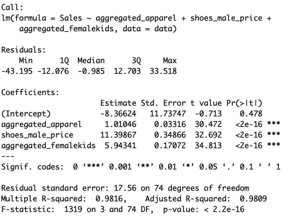
8. As we can see, we get small standard errors now, and the VIFs do look much better:

vif(finalmodel) 

The following screenshot shows the variance inflation factors for the aggregated model: