Putting a specific value for the Bernoulli variables can be viewed as putting a random variable with all its probability mass at 0.5. We could do something slightly more elaborate without making such a strong compromise on the specific value.

Instead of using a fixed value for the Bernoulli variables (0.5), we can use a ka parameter and then put a prior on ka. For example, we can use a beta distribution that is bounded between 0 and 1 (and can be used to generate priors for probabilities, such as our q parameter for a Bernoulli variable). Let's use beta (5,5) random variable. What this means is that, instead of saying that we think with a 100% probability that the proportion of irrelevant variables is 0.5, we are now splitting that 100% into more values. Of course, we are still concentrating them around 0.5 in this case (that obviously depends on the two beta parameters). We could choose any permissible value for those two parameters here, and we would get a different shape:

mod <- " model{
for (i in 1:n){
mu[i] = id[1]*b[1]*x[i,1] + id[2]*b[2]*x[i,2] + id[3]*b[3]*x[i,3] + id[4]*b[4]*x[i,4] + id[5]*b[5]*x[i,5] + id[6]*b[6]*x[i,6]
y[i] ~ dnorm(mu[i], prec)
}
ka ~ dbeta(5,5)
for (i in 1:6){
b[i] ~ dnorm(0.0, 1/2)
id[i] ~ dbern(ka)
}
prec ~ dgamma(1, 2)
}"
jags <- jags.model(textConnection(mod), data = lista, n.chains = 1, n.adapt = 100)
update(jags, 2000)
samps <- coda.samples( jags, c("b","id"), n.iter=1000 )
summary(samps)

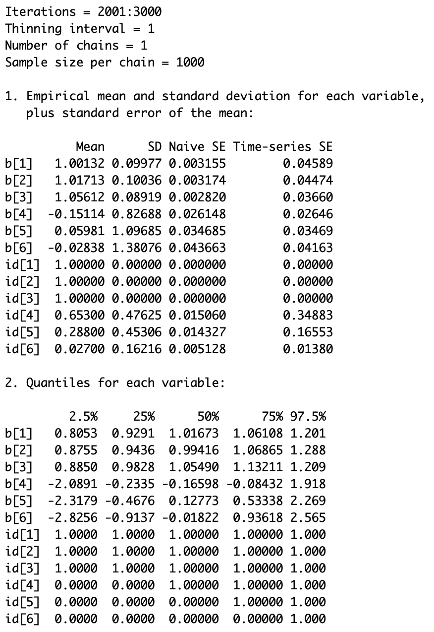
The following screenshot shows the posterior density summary: