Use the following steps to analyze a GLMM:

1. We will use the OrchardSprays dataset, which is included in R. It contains data for an experiment to assess the potency of various constituents of orchard sprays in repelling honeybees, using a Latin square design. The target variable will be a count variable, and the treatment effect will be treatment.rowpos and colpos should ideally be assumed to be random effects. First, we load the libraries:

library(lme4) 
library(emmeans) 
library(MASS) 
set.seed(10) 

2. Let's ignore the random effects and fit this model using the regular GLM framework. Note that we specify family=poisson():

fixed_std_model = glm(decrease ~ treatment,family=poisson(),data=OrchardSprays) 
summary(fixed_std_model ) 

The following screenshot shows the GLM model—all of the effects are fixed:

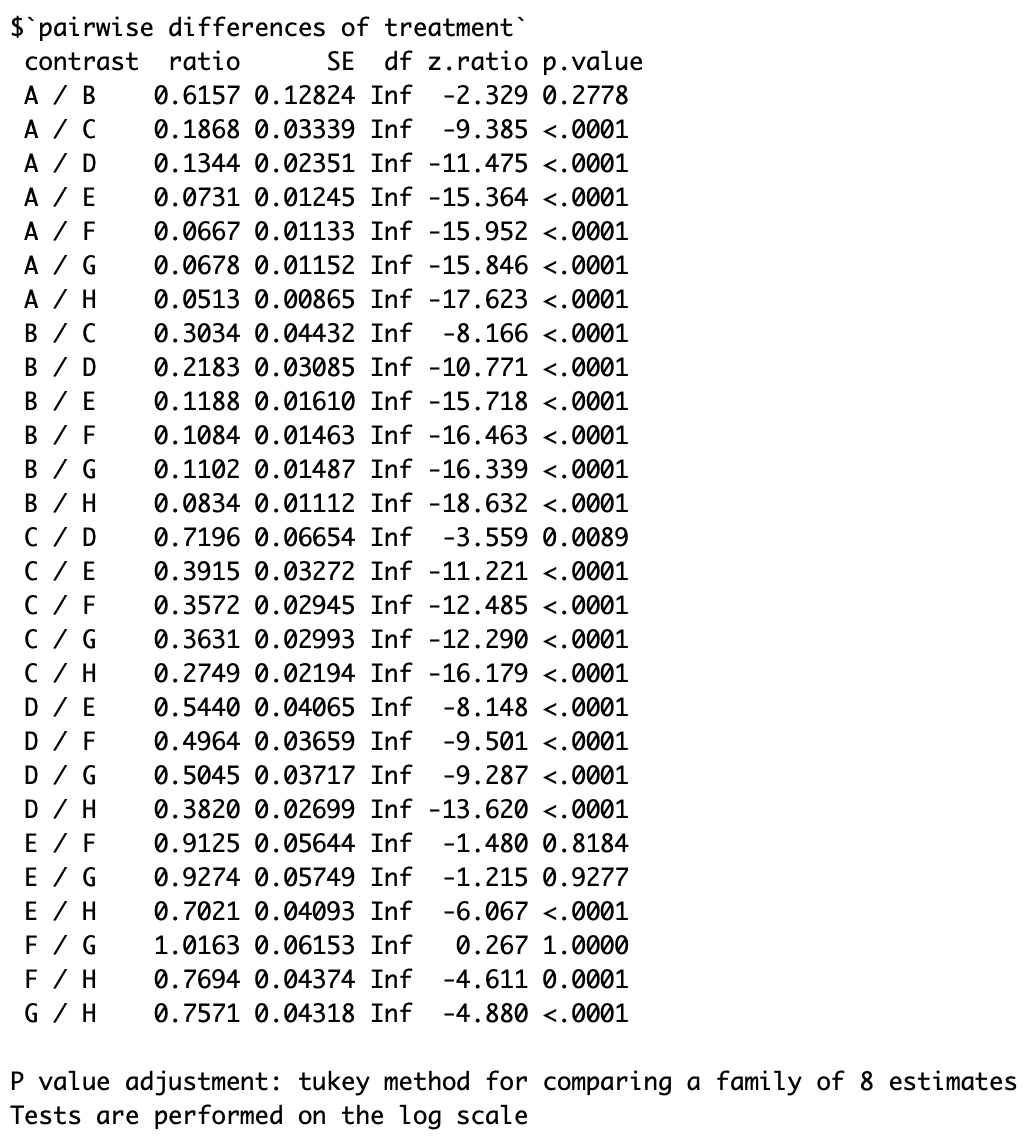
3. We can get the differences between the effects using the emmeans function:

emmeans(fixed_std_model, list(pairwise ~ treatment), adjust = "tukey",type="response" 

The differences between the effects can be obtained using emeans. The Tukey correction is used because we are doing multiple tests. If we do multiple tests using a fixed alpha value of i.e 0.05, the joint alpha will no longer be 0.05 (this is known as the multiple comparison problem):

Take a look at the following screenshot:

4. Predicting is quite easy using the predict function. By default, these predictions will be on the log scale, so in order to force them onto the real scale, we specify type="response":

predict(fixed_std_model,data.frame(treatment="D"),type="response") 

Take a look at the following screenshot:

5. As usual, we can plot the results and check that there is no remaining structure in the residuals. We also need to check that the variance is stable (homoscedasticity). If the residuals are not, then the p-values and confidence intervals will be wrong:

plot(fixed_std_model) 

For the residuals versus fitted values, the variability seems to increase with respect to the predicted values, but we will ignore this issue for the time being:

6. We now incorporate the random effects, and we fit our model using the glmm package. Note that we get a numerical error, meaning that no convergence has been achieved. One possible solution is to rerun the model, but using the previously estimated fixed effects as starting values for the numerical algorithm. Sometimes this fixes these issues, but not always: 

model_1 = lme4::glmer(decrease ~ treatment + (1|colpos) + (1|rowpos), family = poisson(), data = OrchardSprays) 
ss <- getME(model_1,c("theta","fixef")) 
model_2 <- update(model_1,start=ss) 
summary(model_2) 

GLMM model—fixed and random effects on a GLM model:

8. As in standard linear mixed effects models fitted by lmer(), we can get the random effects, the fixed effects, and the variance components:

ranef(model_2) 
fixef(model_2) 
VarCorr(model_2) 

The following screenshot shows the random effects and fixed effects:

9. The residuals should be checked as usual: essentially, we are looking for no remaining structure and constant variance (homoscedasticity):

plot(model_2, resid(., scaled=TRUE) ~ fitted(.) | colpos, abline = 0)
plot(model_2, resid(., scaled=TRUE) ~ fitted(.) | rowpos, abline = 0) 

The following screenshot shows no evident structure is found on the residuals:

The following screenshot shows no evident structure is found on the residuals:

10. We can print, for example, confidence intervals for each effect using the confint.merMod, and we can also get the estimates contrasts using emmeans again:

confint.merMod(model_2) 
emmeans(model_2, list(pairwise ~ treatment), adjust = "tukey",type="response")] 

The following screenshot the 95% confidence intervals:

The following screenshot estimated differences with Tukey's multiple comparison correction: