
7.3. REFERENCES 111
Unknown
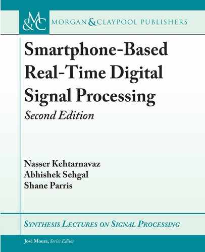
System
Adaptive
FIR Filter
input x[n]
d[n]
y[n]
e[n]
+
Figure 7.1: System identification by adaptive filtering.
where h’s denote the FIR filter coefficients. e output yŒn converges to d Œn. e rate of con-
vergence is governed by the step size ı. Small step sizes ensure convergence at the cost of slow
adaptation rate. Larger step sizes lead to faster adaptation at the cost of overshooting the solu-
tion. Additionally, the order of the FIR filter used limits how accurately the unknown system
can be modeled. A low-order filter will likely not be able to produce an accurate model. Con-
versely, a high-order filter might produce an accurate model but the computational complexity
of such a filter would be prohibitive for real-time operation purposes.
7.3 REFERENCES
[1] J. Proakis and D. Manolakis, Digital Signal Processing: Principles, Algorithms, and Appli-
cations, Prentice Hall, 1996. 110
L7 LAB 7:
IIR FILTERING AND ADAPTIVE FIR FILTERING
is lab consists of two parts. In the first part, the direct form realization of an IIR filter of order
N is compared to its cascade form realization (i.e., N=2 second-order filters). In the second part,
an adaptive FIR filter is used to model or match the IIR filter.
L7.1 IIR FILTER DESIGN
e unknown system that is used as the target for the adaptive FIR filter is an eight-order band
pass IIR filter. e MATLAB function yulewalk is used here to achieve the desired filter design.
Note that the frequency band definitions are decimal numbers ranging from 0 to 1, with 1
..................Content has been hidden....................
You can't read the all page of ebook, please click here login for view all page.