124 8. FREQUENCY DOMAIN TRANSFORMS
1.0
0.8
0.6
0.4
0.2
0.0
Figure 8.3: Hanning window.
stead of processing signal samples in discrete chunks, samples are buffered and shifted through
a time-domain window. Each shift through the buffer retains some of the previous signal infor-
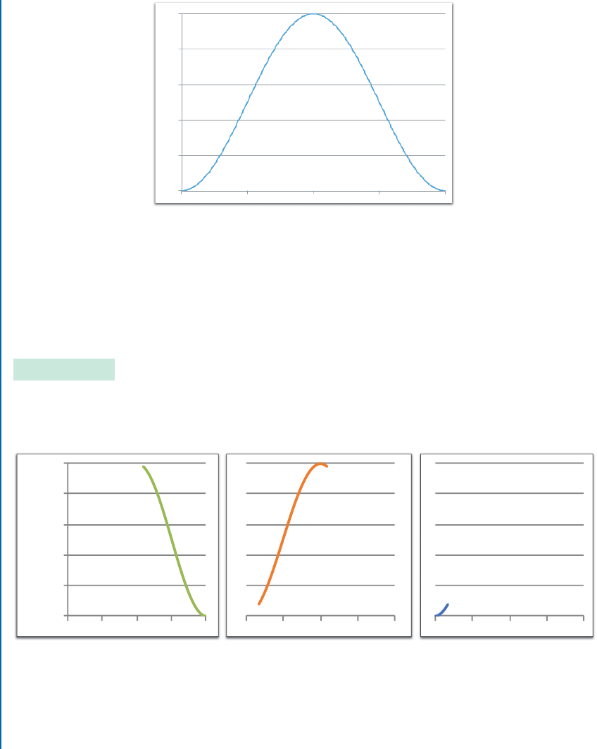
mation, on which the windowing function is applied, as illustrated in Figure 8.4. In this figure,
the input signal is x.n/ D u.n/ u.n 221/ and a Hanning window is generated by calling
Hanning(485) using the C function provided earlier. e frame size, or shift, is considered
to be 221 samples which corresponds to the length of a rectangular pulse. is leads to gaining
greater resolution in the time-domain.
1.0
0.8
0.6
0.4
0.2
0.0
Signal Amplitude
0 121 242 363 484 0 121 242 363 484 0 121 242 363 484
Figure 8.4: Fourier transform windowing (from left to right: iteration 1, 2, and 3).
..................Content has been hidden....................
You can't read the all page of ebook, please click here login for view all page.