7.1 Introduction

Human societies always saw their development strongly tied to energy supplies and the mastering of the processes to exploit them. The growing ability of societies to control and use nature phenomena and resources to improve living conditions, safety, and comfort is always associated to the growth of energy use. Even the quest for more efficient use of energy, in general, just reduces the rate of growth of consumption. This situation today threatens the environment and so poses an immense challenge to humankind as a whole.

Energy, water resources, commodities production, scientific knowledge, and technological expertise are the basis of the development of modern industrial and postindustrial societies.

The recent economic developments implying large-scale industries and inducing large urban concentrations tend to require fairly concentrated energy supplies. Large interconnected systems have been successful in providing these supplies based on thermoelectric plants or hydroelectric generation, wherever there is potential for the latter.

This panorama, however, exerts excessive pressure on primary resources. Fossil fuels are finite and are being consumed at too high rates. A major part of the hydroelectric potentials is already put to use, and most of the remaining potentials are either far away from urban centers or present serious environmental restrictions.

The successive oil crises of the last decades served as incentive for the development of alternative renewable energy sources with lesser environmental impact. Hydroelectric energy has long been an option for micro- and small-scale energy generation. Even in pre-electric times, the water wheel was extensively used as a prime mover. A similar situation is that of wind power, used since ancient times to drive ships and boats, then in windmills and now in wind turbine generators. The direct conversion of solar energy has been a more modern achievement, with heat exchangers and photovoltaic cells. Hydroelectric, wind, and photovoltaic energy sources have reached some technical and economic maturity, becoming the main alternatives in hand.

In specific areas where availability is adequate, geothermal energy is in use. Other types of sources are being studied and shall increase contribution to interconnected systems in great quantities and concentrations such as the oceanic wave, stream, and tide energies.

The main difficulty with systems extensively based in renewable resources is the matching of availability and demand profiles, which are usually quite different. Consumers are too used to burning fossil fuels whenever energy is required. This comfort, available for some centuries now, has deeply marked the relationship between people and energy.

Renewable resources, however, are usually characterized by nonconstant availability profiles. It is usually unlikely that the resource will be available when required, and it is not reasonable nor even feasible to try to concentrate demand when the resource availability is greater.

One way to face source scarcity periods while keeping energy costs down is using two or more different energy sources in hybrid systems, at the expense of higher initial investments. This allows the use of, say, two sources with smaller conversion/storage devices in the system than would be necessary if only one of the sources was used, while still improving supply failure avoidance.

In the last few years, many feasibility studies have been concentrating on systems based on wind and photovoltaic power, with the possible support of diesel-driven generators. Hydropower is frequently considered for support in these types of systems, due to its usually more regular availability. In these systems, energy storage is always fundamental to warrant demand satisfaction during scarcity periods.

A characteristic worth considering is the possible complementarity of availability among the sources considered. A hybrid system based on two different sources may profit from their complementary availability throughout a period of one year. In the season when one source is scarcely available, the other would be mainly in charge of the supply, while in the other half-year the situation would be reversed. It is possible to devise adequate ways of sizing the powers of the conversion devices and the capacities of the energy storage equipment for use under this new conception.

This notion of complementarity opens new perspectives for ideas related to the design of hybrid systems. Given some site or region, the complementarity potentials of the existing resources are usually measurable. Complementarity data are sort of an information support for energy resource managers, useful for the ranking of energy generation projects and/or devising an energy supply strategy for a region. On a lesser scale, for independent entrepreneurs, complementarity may be related to circumstantial opportunities arising from the availability of energy resources or specific equipment, or even from the needs or creativity of the concerned engineer or investor.

This chapter studies energy-complementarity by describing types, establishing the definition of perfect complementarity between two types of sources and presenting a method for the analysis of the performance of a hybrid system. This analysis seeks to evaluate performance as a function of the different degrees of complementarity between the contemplated sources. Some comments on the effect of energy accumulators on the performance of this type of system are included. This chapter also presents some practical cases where feasibility was evaluated for real systems based on partially complementary resources.

7.2 Energetic Complementarity

Complementarity can be seen as the property of one or more energy sources to complement each other's production over a certain space and/or over time intervals. At this point, a better understanding of energetic complementarity and how to evaluate the different degrees of complementarity in time or space is required.

Space-complementarity may exist when the energy availabilities of two or more types of sources complement themselves within a certain region. An example (McVeigh, 1977) is the complementarity between solar and wind resources over the territory of Great Britain, which is scarcely exploited due to the small amounts of energy available.

Time-complementarity may exist when the energy availability of two or more types of energy resources present periods of availability that are interlaced over time in the same region. An example is the complementarity in time between hydro and solar resources throughout the State of Rio Grande do Sul in southern Brazil, characterized by Beluco et al. (2008a,b).

Complementarity may also exist when the availability of energy of only one type of source is considered in different parts of a vast region and over time. As an example, the availability of hydraulic energy over the Brazilian territory (Damázio et al., 1997) may be mentioned, as this was one of the main reasons for interconnecting the south-southeast and the north-northeast electrical energy supply systems. This is an example of complementarity in time and space.

Different energy availabilities may be considered perfectly complementary if the variation of the availability values presents equal periodicity and their respective maximum and minimum values occur in time intervals half a period apart (out of phase). Furthermore, the average values of the availabilities should be the same, as well as the relation between the respective maximum and minimum values of availability of the two sources.

The amounts of energy supplied by generators in a hybrid system are considered complementary in time, even when the availability values are not perfectly complementary. The availabilities may present an imperfect complementarity, and the generators may be sized to supply energy values having the same average throughout the period. Obviously, this is possible only if the available energy is greater than the energy in demand.

Figure 7.1 presents two sinusoidal curves, showing a complementary instance, which will be considered perfect for the purposes of the present work. The two curves present hypothetical availabilities of two sources of energy, expressed in terms of energy or power throughout a year.

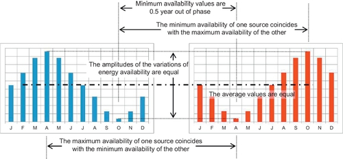
Both curves present periods of one year, average values equal to 1, maximum values equal to 1.2, and minimum values equal to 0.8. The minimum of the first curve occurs at 0.75 of the year, whereas the one of the second curve is at 0.25 of the year, or 0.5 year out of phase.

The complementarity between these curves is considered perfect because the minima and the maxima are 0.5 year out of phase, the difference between the maximum and the minimum is 0.5 in both cases, and the average values are equal.

The functions depicted in the figure may represent energy availabilities of two sources or the energy or power supplied by two generators. These functions will be used for the setup of a complementarity index, but they do not adequately describe, in detail, the behavior of solar sources, for example, because these present daily variations have an effect on the detailed behavior of hybrid systems.

The need to evaluate how much two availability functions, which are not perfectly complementary, differ from the situation depicted in Figure 7.1 (considered as a reference) naturally leads to the creation of numerical dimensionless indexes considering the aforementioned characteristics. Indexes varying from 0 to 1 are suggested to evaluate the complementarity in time between, for instance, hydraulic and solar energy availabilities.

7.3 Evaluation of Complementarity in Time

Among the types of complementarity previously discussed, this section is dedicated to complementarity in time. The article of Beluco et al. (2008a) proposed a dimensionless index evaluating different degrees of complementarity. An index created in this way should be seen as a tool that can be molded according to the decisions to be taken.

The complementarity index, 6, necessarily involves time and is designed to express the degree of complementarity between two energy sources. It is defined according to Equation (1) and includes the evaluation of three components: the phase difference between the energy availability values of the two sources, the relationship between the two average availability values, and the relationship between the amplitudes of variation of the availability functions.

$\kappa ={\kappa }_t{\kappa }_e{\kappa }_a$

In this equation, κ_t is the partial time-complementarity index reflecting the phase difference, κ_e is the partial energy-complementarity index describing the complementarity between the average values of energy availability, and κ_a is the partial index of amplitude-complementarity taking care of the relation between amplitudes of the variation of the energy availability of the sources.

The partial index κ_t is defined by Equation (2) and measures the effect of the time interval between the minimum values of availability of the two sources of energy. If this interval is exactly half the period, the index will be equal to 1. If the interval is null (i.e., if the availability minima coincide), the index will be equal to 0. Intermediate values are linearly related.

${\kappa }_t=\frac{\left|d_{\mathrm{h}}-d_{\mathrm{s}}\right|}{\sqrt{\left|D_{\mathrm{h}}-d_{\mathrm{h}}\right|\left|D_{\mathrm{s}}-d_{\mathrm{s}}\right|}}$

In this equation, D_h is the number of the day of the maximum value of hydraulic energy availability, d_h is the number of the day of the minimum value of hydraulic energy availability, D_s is the number of the day of the maximum value of solar energy availability, and d_s is the number of the day of the minimum value of solar energy availability. This expression may be rewritten as Equation (3), supposing that the respective (D− d) differences are equal to half a year, which is more practical for estimates.

${\kappa }_t=\frac{\left|d_{\mathrm{h}}-d_{\mathrm{s}}\right|}{\sqrt{180\times 180}}=\frac{\left|d_{\mathrm{h}}-d_{\mathrm{s}}\right|}{180}$

The partial energy-complementarity index κ_e is defined by Equation (4). It evaluates the relationship between the average values of the availability functions. If the average values are equal, the index should equal 1. If those values are different, the index should be smaller and tend to 0 as differences increase. Intermediate values of difference are linearly related to the index.

${\kappa }_e=1-\sqrt{{\left(\frac{E_{\mathrm{h}}-E_{\mathrm{s}}}{E_{\mathrm{h}}+E_{\mathrm{s}}}\right)}^2}$

In this equation, E_h is the total of the hydraulic energy over the year and E_s is the total solar energy over the same period.

Alternatively, an expression for κ_e may be developed from a coefficient e as defined by Equation (5). This coefficient varies between 0 and 2, being equal to 1 when energies E_h and E_s are equal. When E_h is much bigger than E_s, e tends to 2, whereas if E_h is much smaller than E_s, e tends to 0.

$e=\frac{2}{1+\frac{E_{\mathrm{h}}}{E_{\mathrm{s}}}}$

The index κ_e, however, should be κ_e = 0 if e = 0 or e = 2 and κ_e = 1 when e = 1. This is obtained by Equation (6), which is equivalent to Equation (4).

${\kappa }_e=1-\sqrt{{\left(1-e\right)}^2}$

The partial amplitude-complementarity index κ_a is defined by Equation (7) and evaluates the relationship between the values of the differences of the maxima to the minima of the two energy availability functions. If those differences are equal, the index shall be equal to 1. Otherwise, the index shall fall from 1, tending to 0.

${\kappa }_a=\left\{\begin{array}{l}\left[1-\frac{{\left({\delta }_{\mathrm{h}}-{\delta }_{\mathrm{s}}\right)}^2}{{\left(1-{\delta }_{\mathrm{s}}\right)}^2}\right],\mathrm{f}\mathrm{o}\mathrm{r}{\delta }_{\mathrm{h}}\le {\delta }_{\mathrm{s}}\hfill \\ \left[\frac{{\left(1-\delta \right)}^2}{{\left(1-{\delta }_{\mathrm{s}}\right)}^2+{\left({\delta }_{\mathrm{h}}-{\delta }_{\mathrm{s}}\right)}^2}\right],\mathrm{f}\mathrm{o}\mathrm{r}{\delta }_{\mathrm{h}}\ge {\delta }_{\mathrm{s}}\hfill \end{array}\right.$

This index is obtained from a suitable manipulation between the δ_h and δ_s, the differences between the respective maximum and minimum values of the energy availabilities. These differences are obtained from Equation (8), where E_d max is the maximum daily energy availability value in a year, E_d min is the minimum daily energy availability value in a year, and E_d c is the annual average daily energy consumption.

$\delta =1+\frac{E_{\mathrm{d}\max }-E_{\mathrm{d}\min }}{E_{\mathrm{d}\mathrm{c}}}$

This index was created to include the difference between the maximum and the minimum energy availability of the sources in the complementarity evaluation. If one of the sources has no available energy throughout the period of interest, it is impossible to consider it for complementarity purposes. If the two sources have the same difference between maximum and minimum availability, they are ideally amplitude complementary and the index should be equal to 1. In the intermediate cases where the differences are unequal, the index should express it by values between 0 and 1 for less-than-ideal complementarity.

The δ_s difference is always greater than 1 and may be considered constant over quite an extensive area because it represents the availability of solar radiation. The δ_h difference presents a minimum value of 1, in which case the complementarity index should be null. On the other hand, δ_h may present rather large values as compared to δ_s, and in these cases, the index should decay from the maximum value as the δ_h value increases.

For the purpose of the development of the expressions for the κ_a index, described in the next few paragraphs, the value δ_s = 2 was considered. The resulting curve shall be continuous and smooth, it shall present a zero slope for δ_h = δ_s, and it shall be very nearly symmetrical in the proximity of its peak. It is also desirable to obtain an expression for the quick calculation of the κ_a index. The desired behavior for this function is shown in Figure 7.2.

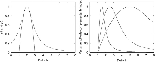
There is no obvious mathematical expression for a function with those characteristics. The development of an expression for the part of the curve to the right of the maximum can be based on the Agnesi curve, adapted so that its maximum value is 1 and corresponds to an abscissa equal to δ_s, which leads to Equation (9).

$y_2=\frac{1}{1+{\left({\delta }_{\mathrm{h}}-{\delta }_{\mathrm{s}}\right)}^2}$

The Agnesi curve presents the desired symmetry characteristics with respect to its maximum for the abscissa δ_h equal to δ_s. The final form for the right side of the function is obtained by slightly modifying Equation (9) to smooth the slopes near the maximum, to ease its connection to the expression to be used for the left part of the curve in Equation (10).

$y_2=\frac{{\left(1-{\delta }_{\mathrm{s}}\right)}^2}{{\left(1-{\delta }_{\mathrm{s}}\right)}^2+{\left({\delta }_{\mathrm{h}}-{\delta }_{\mathrm{s}}\right)}^2}$

For the left part of the curve, a quadratic function seems adequate in view of the three contour conditions. The y₁ function, with δ_h as the independent variable, centered in the value of δ_s, is presented in Equation (11).

$y_1=1-\frac{{\left({\delta }_{\mathrm{h}}-{\delta }_{\mathrm{s}}\right)}^2}{{\left(1-{\delta }_{\mathrm{s}}\right)}^2}$

Figure 7.2(a) shows the superposition of the curves y₁ in solid line and y₂ in dotted line. Figure 7.2(b) shows three different curves' amplitude-complementarity index, for δ_s values of 1.5, 2.5, and 5.

7.4 Complementarity Between Solar Energy and Hydropower

This section is dedicated to complementarity between solar and hydroelectric energies, and discusses the determination of the proposed index in real conditions.

The calculation of complementarity indexes for large regions can provide an important tool for managers of energy resources. For example, the application of funds for electrification of a region can be decided based on the existing complementarity, because generation systems based on complementary resources may have less installed power.

The climatic conditions in southern Brazil promote the notion that higher rainfall occurs during periods of reduced insolation and, conversely, that lower rainfall occurs during periods of intense sunlight. This notion is the origin of this study, starting with the possible complementarity between solar energy and hydropower. It seeks understanding of its effects on hybrid generation systems based on these resources.

In a real situation, the calculation of the indexes may be carried out through functions adjusted to the monthly average data by the least squares method. Figure 7.3 shows monthly average precipitation data and monthly average of daily incident solar radiation data over a flat horizontal surface, as supplied by a weather station in the state of Rio Grande do Sul (FEPAGRO, 1989).

The solar energy availability in Figure 7.3 is quite similar to the idealized curve of daily availability shown in Figure 7.1. The situation is different for the water availability, a second lesser peak appearing near the position of the valley of the idealized curve.

The monthly average precipitation does not adequately represent the water availability. However, in smaller river basins, flow variations present small phase lag with respect to precipitation variations, and the amplitudes of the variations are also closely related. The water availability curve is lower in the January-May interval. If January is used, because the minimum solar availability is in July, the partial time-complementarity index is equal to 1.00. The partial energy-complementarity index and the partial index of amplitude-complementarity evaluations are not possible using these numbers. However, an expedited evaluation is made to allow the elaboration of the maps that follow.

The determination of the indexes from river flow data may be done in the same way, using adjusted curves over the monthly average data. The use of daily data for water and solar availability would certainly produce better results!

The value of δ_s used for this work is 1.2860. The value for δ_h may vary considerably as a function of the water availability in the plant area and the installed capacity of the hydroelectric generator. Moreover, considering its definition, δ_h will never be less than 1, which corresponds to the hydroelectric generator always turning out the same power and the corresponding flow presenting a short recurrence time, which implies a high frequency.

The calculation of these indexes for the entire state of Rio Grande do Sul in southern Brazil allows mapping. Beluco et al. (2008a) shows these maps for the partial indexes and the overall index. The systems based on the availabilities with the higher time-complementarity (which can be evaluated from the indexes proposed here) tend to present fewer consumer demand satisfaction failures. So, from this point of view, the complementarity map shows the “best” areas for the use of hydraulic and solar complementary availability.

Figure 7.4 shows the map of complementarity in time for the State of Rio Grande do Sul. This is one of the maps presented by Beluco et al. (2008a). The information that appears in Figure 7.3 was determined from a database of the Agricultural Research Foundation of Rio Grande do Sul (FEPAGRO, 1989, 2000). From this same database, data from 15 weather stations (including Taquari) were used for preparing the map that appears in Figure 7.4.

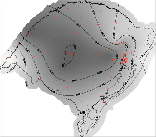
In areas where the time-complementarity index is less satisfactory, the complementarity condition can be helped by the use of water reservoirs, with the effect of improving the phase difference between the minima to near a half-year, which is the ideal value. Regions with a smaller κ_t will require bigger accumulation volumes for the system to approach the performance levels corresponding to a full complementarity. In this sense, a photovoltaic hydroelectric system can be supported in a more natural way with stored energy in water reservoirs and batteries.

In the same way, small differences in the amplitudes of variation of the hydraulic and solar availabilities also lead to better performing systems. The map of complementarity between amplitudes shows the best-valued areas for the amplitude-complementarity index that are, consequently, the best areas (from this point of view) for consumer demand satisfaction.

In areas with lower values for this index, the generating systems' performance can also be improved by the use of reservoirs. This can help improve the amplitude variation of the hydraulic availability approaching it to the value corresponding to the perfect complementarity, which is the same as the variation of the solar availability. And, as previously mentioned, regions with a smaller index value will need bigger reservoirs for a given level of system performance.

The complementarity maps presented by Beluco et al. (2008a) indicate that about 58% of the area of the state has a κ_t greater than 0.60, corresponding to more than 72 days of phase difference between the minima of the two availability curves, the best values occurring from the southeast to the northwest border. It can also be seen that nearly 50% of the state area presents κ_t values greater than 0.80, that is, phase differences of nearly 50% of the cycle of the hydraulic and solar energies' availability, the extreme values appearing in the center of the state. On the other hand, 4.67% of the state area presents κ values greater than 70%. It is, however, clearly visible that the most adequate area from the time-complementarity point of view is generally not the most adequate area from the amplitude-complementarity point of view. The final complementarity index κ will consequently show intermediate values in these areas, whereas the best values will be near the northwest border.

A precise and reliable evaluation of complementarity in a given place should be based on flow data across a given river section and on incident solar radiation data taken daily. The insight on the hybrid system performance gained through computer simulations and experimental studies allows the evaluation of the effects of the complementarity on the system parameters and may justify deeper and more comprehensive studies for the characterization of the complementarity.

7.5 Hydro-PV Hybrid Systems Based on Complementary Energy Resources

A hybrid hydro-photovoltaic (PV) plant is a generation system based on a hydroelectric plant and a photovoltaic plant operating together to satisfy the demand of an ensemble of consumer loads. The complementarity between the energy sources may then be beneficial for the sizing and the operation of this type of system. The International Centre for Application of Solar Energy (CASE, 1997) describes the installation of a hydro-PV system in Ban Khun Pae, north of Thailand, comprising 60 120 Wp modules, a 90 kW synchronous generator, batteries with 110 kWh storage capacity, a 40 kW inverter, and a 56 kW diesel backup unit. The hydroelectric plant was preexistent but insufficient to supply the needs of the population of about 90 dwellings. The cost of this system was approximately $170,000. The use of PV modules was considered for supplementing the existing hydroelectric system, but the reference does not discuss the idea of complementarity.

The state of charge of the various storage devices may be managed according to the chosen operation strategy, which shall include the consideration of the effects of complementarity between the energy sources. The chosen operation strategy may contemplate the action of the battery bank to attenuate electromechanical transients in the turbine-generator system, because time constants of electrical transients are much smaller than those of mechanical transients. Van Dijk et al. (1991) suggests an increase in battery life by using 90% of full capacity as the recharge level.

If a direct current (DC) hydroelectric generator is used or the generator current is rectified and the consumer loads accept DC, only a DC bus is necessary. However, because alternating current (AC) hydroelectric generators are more common, two busses are necessary, as depicted in Figure 7.5. In this type of system, the current from the hydro generator is tied to the PV generator, the batteries, and the loads through the DC bus. A regulator may manage the connection and disconnection of generators and loads to the batteries as a function of the state of charge of the latter and define the current level to be supplied by the hydro generator. This configuration is quite usual for systems based on renewable sources, as it is a simple alternative for conditioning the power supplied by induction generators. For this configuration, in case the hydro plant is equipped with induction generators, the rectification avoids the need for a tight frequency control. The voltage regulation may be simplified or even omitted, with the excitation being handled simply by a capacitor.

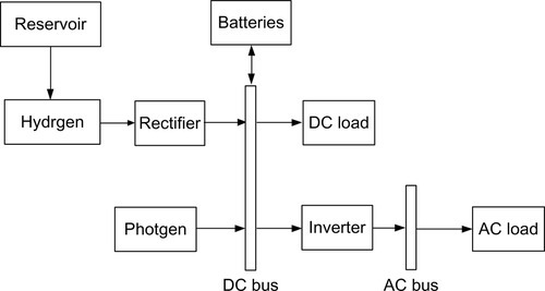
Those systems are suitable for demands of a few kilowatts. A 24 V DC bus for 1-2 kW will handle currents of the order of 40-80 A. On the other hand, a battery bank at 127 V, allowing greater powers with smaller currents and comparable storage capacity, using automotive batteries would have an exaggerated size. Automotive batteries may be replaced with a technical and perhaps economic advantage by lead-acid stationary batteries. Automotive batteries are supposed to work under a certain level of vibration.

The system depicted in Figure 7.6 is much more complex, involving the parallel operation of an AC generator and a power-converting device. In such a system, the AC bus frequency may be easier to regulate if it is the frequency of the hydro generator when this machine is in use. If a synchronous generator is used, the inverter can operate at an approximately constant frequency, equal to that of the generator. If an asynchronous machine is used, the inverter may operate on a variable frequency following the instantaneous values of the generator frequency. In such a configuration, it may be possible that the control of the inverter frequency, in certain conditions, may allow some control of the generator frequency and, consequently, of the bus frequency.

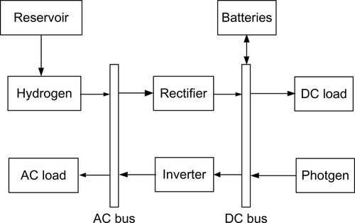
This type of system does not have power limitations. The DC bus currents will certainly be the highest currents supplied by the PV modules. In the AC bus, the voltages can be higher and defined by the hydro generator.

If the hydro and solar energy availabilities are time-complementary, the storage devices may be sized to optimize the operation of the hybrid system. The water reservoir may be sized for a shorter period, implying lower costs and lesser environmental impacts if the hydroelectric generator operates with a photovoltaic generator and a battery bank, provided there is a complementarity between the two energy sources.

It is possible to define an operational strategy for a hydro-PV system as follows: (1) use all the energy provided by the PV generator, polarized by the battery bank voltage (which is determined by its state of charge); (2) operate the battery bank in intermediate charge states (when it has a relatively good capacity for either charge or discharge) to attenuate electromechanical transients due to variations in the sources or in the load; (3) store energy in the water reservoir and in the battery bank, their state of charge being managed as a function of the energy availabilities and energy demand, while considering the possible complementarity of the sources; and (4) operate the hydro generator to address the consumer loads not attended by the PV generator, while considering the states of charge of the storage devices.

7.6 A Method of Analysis

It is necessary to know how a hybrid system based on complementary resources will have its performance influenced by the complementarity of the energy resources. Beluco et al. (2012) propose a method of analysis that has as its starting point the idealization of the available energy. A hybrid system could be simulated with real data, but the results would be subject to the climatological effects. The simulation using idealized data, such as that appearing in Figure 7.1, allows an accurate assessment of the effects of complementarity on the performance of the simulated system.

In this sense, the results of simulations performed with idealized data can be viewed as an upper limit of the simulated system performance. This theoretical limit would be setting an unattainable performance in real conditions. This “maximum performance” would be obtained with the maximum energy that could be available from a certain source if this source were insensitive to random events typical of the environment and insensitive to periods of extreme energy scarcity or extreme availability.

A theoretical limit of performance may be determined from a simulation of a power plant for a year of operation based on functions of energy availability synthesized specifically to this end. These functions may be synthetic series of data obtained from real energy availability data or they can be mathematical functions (such as a sinusoid) with parameters extracted from the series of real data. A further step in the analysis can obviously be the comparison of these results with those obtained with the actual data.

The performance of an energy generation plant may be evaluated by the total of the supply failure times (SFT) observed during a given elapsed time, or by a supply failure index, F, defined as the SFT divided by the corresponding elapsed time. A failure is defined as any situation where the total power supplied by the energy conversion devices is less than the power required by the consumer loads. A failure occurs also if, besides insufficient power, there is no stored energy available for consumption. The elapsed time considered in the analysis may be given in days, weeks, months, seasons, or years.

The failure index is adopted as the performance evaluating parameter and theoretical limit of performance for given operational conditions and energy availabilities. The performance of a power plant will be better as the failure index is smaller and the power or energy required by consumers and effectively supplied by the system is bigger. The upper limit for the failure index is the null index, meaning that all the demand was satisfied, and it may even happen that excessive energy is being offered.

In this chapter, this method was applied in order to obtain some information regarding the effects of complementarity on the performance of hybrid systems based on complementary energy resources. The final part of this section will describe how simulations based on this method were performed. After that, the next section will present some results for the theoretical limit of performance. Then, the following section will present the results obtained for some real cases, simulated with the Homer software.

The hybrid system under study was simulated on the computer with the objective of investigating its performance and subsidizing the establishment of technical bases for a sizing methodology, with special regard for the various degrees of complementarity between the availabilities of the energy resources used. The simulations were made with routines written with MATLAB (MathWorks, 1999). The program simulates the system depicted in Figure 7.6. The values of 0.68 and 0.175 are adopted for the efficiencies of the hydro and PV generators, respectively.

The input to the simulation program consists of information on the yearlong energy availability of the sources used and of the sizes of generators and storage devices. The output is a report on the supply of the demand of the load during the simulation period. Basically, the total of the SFT is evaluated.

The program adopts the per unit (pu) in which the variables are made dimensionless with respect to an outstanding value (typically a reference design value or a nominal value), and it simulates the plant behavior during a two-year time interval without consideration for transient effects. The output file contains hourly records of the system components during the second simulated year, the calculations being repeated every five minutes, with the objective of reducing the influence of the storage devices' initial states on the final results of the simulation.

The total instantaneous power available to the hydroelectric generator is simulated in a theoretical way, using a sinusoidal function. The energy availability represented by this function depends on the location chosen for the hydroelectric plant and may present considerable variation in amplitude and in annual energy availability.

The total instantaneous power available to the PV generator is simulated by three functions. The first one describes the availability during each day; the second one describes the maximum daily availability throughout the year, and the third one, the variation of the duration of the day throughout the year. These functions are not based on the typical equations developed for the description of solar irradiance such as, for example, those presented by Duffie and Beckmann (1980), but they are similar to the function describing hydro availability throughout the year.

The maximum and minimum average values for the total instantaneous power available to the photovoltaic generator were obtained from monthly data as published by FEPAGRO (1989). The pu values of 0.67783 (corresponding to an incident solar radiation of 677.83 W/m²) and of 0.37108 (corresponding to an incident solar radiation of 371.08 W/m²) are considered for the respective maximum and minimum instantaneous power available to the PV generator.

The demand profile, p_L, considered in the simulations corresponds to a constant energy consumption throughout the day. Other profiles may be used, such as profiles with a concentration of consumption during the day or with a consumption peak at the end of the afternoon.

Figure 7.7 shows the result of the simulation of a system with total complementarity and the battery bank sized for two days' storage. The horizontal axis is time in years, while in the vertical axis various functions are represented: to the left are the scales for the powers supplied by the generators and consumed by the load; to the right is the state of charge of the batteries (SOC).

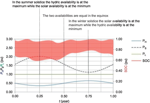
The line above, forming a spot shows the SOC. The gray line below represents the hydropower supplied (p_H), the black dashed stands for the maximum daily PV power (p_P max d), and the most thin gray is the power consumed by the loads (p_L). It can be seen that there are no shutoffs of the hydroelectric generator and no supply failures.

In the simulated system, the annual energy available for consumption is equal to the annual energy demand, and also the system has a complementarity index equal to 1 (κ = 1.00), which means perfect complementarity. Consequently, the time-complementarity index, κ_t, the energy-complementarity index, κ_e, and the amplitude-complementarity index, κ_a, are also equal to 1 (κ_t = 1.00, κ_e = 1.00, κ_a = 1.00).

If, for example, the system has loads consuming a constant 600 W of power, the hydroelectric generator should have a minimum 534 W of installed power and the PV generator should use 16.40 m² of collector area. The daily consumption is then 600 Wd or 14,400 Wh, and the battery bank should have a capacity for double that (28,800 Wh). This storage capacity may be obtained by 8 150 Ah 24 V batteries.

In Figure 7.7, it can be seen that the maximum hydroelectric power supplied by the generator is equal to 0.89, which, for the example given, means 534 W. It is interesting to note that this power is 11% smaller than the power required by the loads. In small systems such as the one considered in the example, such an advantage is difficult to materialize due to the standardization of equipment commercially available.

The dimensionless area of the PV modules, a_P, is 17.69, as calculated by Equation (12) and indicated in the caption for Figure 7.7, where A_P is the area of the PV modules and P_{L max} is the reference value for power. In the example, this area is equivalent to 16.40 m² and may be obtained with 16-18 commercial 1 m² modules on the market. This area will provide about 1500 Wp of power, where the maximum PV availability is around 2.50 pu.

$a_P=\frac{A_P}{\left(\frac{P_{L\max }}{1000}\right)}$

The system of Figure 7.7 was considered the “starting point” for the simulations, a reference for easy comparisons with the results presented. The choice was made based on comparisons among different proportions between the total annual energy available for consumption and the total annual energy required by the loads.

The hybrid system under study, sketched in Figure 7.6, was simulated on the computer with computational routines written with MATLAB, as described in Equation (5). The simulations adopt the pu system to describe the physical quantities, where each quantity is divided by a reference value associated with the dimensions of each component of the system or with the reference values of available energy or demand.

The operational strategy: (1) Use all the energy provided by the PV generator; (2) operate the batteries in intermediate charge states; (3) store energy in the water reservoir and in the battery bank, their state of charge being managed as a function of the energy availability and demand while considering the possible energetic complementarity; and (4) operate the hydro generator to address the consumer loads not attended by the PV generator, while considering the states of charge of the storage devices.

The operation of the hydro generator is obviously different from the usual operation of a hydroelectric power plant, but it should be clear that a system like the one proposed in this work should be focused on better utilization of available power and simplicity of control.

The theoretical limit of performance (Beluco et al., 2013b) is defined as the upper limit for the performance of a power plant corresponding to the performance obtained with the “maximum availability” of the energy resource. This would be the maximum energy that could be available from a certain source if it were insensitive to random events typical of the environment and insensitive to periods of extreme energy scarcity or extreme availability.

The maximum and minimum average values for the total instantaneous available power to the PV generator are obtained from monthly data for the region considered in this study. The pu values of 0.67783 (corresponding to an incident solar radiation of 677.83 W/m²) and of 0.37108 (corresponding to an incident solar radiation of 371.08 W/m²) are considered for the respective maximum and minimum instantaneous power available to the PV generator.

The simulated system is designed from the proportions between the total annual available and demanded energies (π_ad); the total annual available hydro and solar energies (π_sh); and the difference between the maximum and the minimum availabilities (π_Mm), as defined by Equation (13). For a constant demand profile, the power required by the loads is considered equal to 1. The available hydro and PV powers are defined as a function of the aforementioned proportions and present sinusoidal variations throughout the year.

${\pi }_{\mathrm{ad}}=\frac{E_{\mathrm{s}}+E_{\mathrm{h}}}{E_{\mathrm{d}}}{\pi }_{\mathrm{s}\mathrm{h}}=\frac{E_{\mathrm{s}}}{E_{\mathrm{h}}}{\pi }_{\mathrm{ad}}=\frac{{\delta }_{\mathrm{s}}-1}{{\delta }_{\mathrm{h}}-1}$

For a constant demand profile, the power required by the loads is considered equal to 1. The available hydro and PV powers are defined as functions of the aforementioned proportions and present sinusoidal variations throughout the year.

Figure 7.7 shows the result of the simulation of a system with total complementarity and the battery bank sized for two days' storage. The horizontal axis is time in years, while in the vertical axis various functions are represented: to the left are the scales for the powers; to the right is the SOC. The line above, forming a spot shows the SOC; the gray line below, the hydroelectric power supplied (p_H); the black dashed line, the maximum daily photovoltaic power (p_P); and the most thin gray, the power consumed by the loads (p_L). It can be seen that there are no shutoffs of the hydroelectric generator and no supply failures.

This system was considered the “starting point” for the simulations, a pattern for easy comparisons with other results. The choice was made after a survey of different combinations of components and their importance for achieving the expected results.

The results presented by Beluco et al. (2012) showed a slight difference in relation to the system of Figure 7.7. Results of that paper clearly show the energy stored in the batteries, with two peaks over a year. The two simulated systems show small differences and, because of that, this result did not appear in Figure 7.7. This behavior of the batteries is being studied, and the results characterizing the transition from the system will be published soon.

The study of the effect of different degrees of complementarity on the performance of the energy system considered is based on the effects of the variations in the energy availability and of different combinations of installed power of hydro and of photovoltaic generator sets, in addition to the effects of the range of water discharges turning the hydroelectric generator.

7.7 Effects of Complementarity in Time

Complementarity can be verified over space and time, as previously mentioned. It is a topic that still has many details to be discovered. This section presents some basic results about the influence of complementarity in time on the performance of a hydroelectric-photovoltaic hybrid system, according to the proposed method of analysis.

7.7.1 Effects of Different Degrees of Complementarity in Time

The system for which simulation results are depicted in Figure 7.7 has a perfect complementarity, with total annual energy available being equal to the total annual energy required by the loads, the battery bank having a 24-hour capacity with discharge to 40% and recharge to 100% of full capacity, and without a reservoir. It does not show any demand satisfaction failures.

The use of idealized data brings out various aspects of the performance of hydro-PV systems running on complementary energy resources. This procedure helps define the applicability of the system and supports the sizing of its components. The configuration of this system is not necessarily a “target configuration” for sizing purposes, but it is the most valuable source of information on the performance of this type of system.

When complementarity is less than perfect, variations in performance as functions of partial indexes being less than 1.00 will be observable. As time-complementarity index κ_t varies, characterizing poorer complementarity, performance degrades and failures may appear, as shown below. A worse time-complementarity, as seen in Figure 7.8, is associated to higher failure indexes. Values of κ_t equal to 0.8333, 0.6667, 0.5000, and 0.0000, respectively, resulted in F values of 0.0670, 0.1041, 0.1383, and 0.1758.

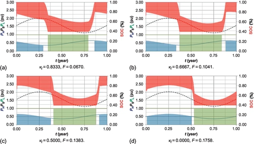
Figure 7.9(a) details the period between the 89th and 93rd days, showing the shutdown of the hydroelectric generator during the period of intense sunlight. Figure 7.9(b) details the period between the 287th and 291st days, showing the failure in meeting demand due to energy shortages.

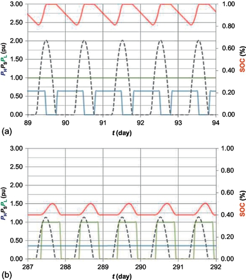
These results explain the dark gray, light gray and medium gray spots that appear in the graphs, corresponding respectively to the hourly fluctuations of the SOC, the power supply failures and periods of surplus energy, and consequent shutdown of the hydroelectric plant.

A reservoir may artificially improve time-complementarity, having the effect of delaying the low hydro availability period. The value of the failure index may imply an initial value for the required reservoir volume, and is strongly related to the conditions of the plant location.

The reservoir design may aim at improving complementarity characteristics, causing imperfect natural complementarity to improve, and to approach a situation leading to a better operation of the hydro-PV hybrid system.

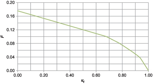
Figure 7.10 summarizes the results of Figure 7.8 and shows the variation of failure index F with the complementarity in time.

7.7.2 Effects of Different Degrees of Energy-Complementarity

The effects of variations in the energy-complementarity index are depicted in Figure 7.11, the graphs being obtained in the same way as in Figure 7.8. The values of the ratio π_sh, the index κ_e, and the results for F are listed in the legend of each result. Four results are shown, corresponding to the values of 1.43, 1.67, 0.70, and 0.60 for the ratio π_sh, and the values of 0.8275 and 0.7500 for the κ_e index. For reference, the system of Figure 7.7 has unity values for π_sh and κ_e.

The values of π_sh imply different average energy availabilities. For the first two results, the photovoltaic energy supplied tends to increase, while the supplied hydropower tends to decrease. Because the solar availability presents great daily and yearly variations, when its relative importance increases, so does the failure index. These variations cause corresponding, however subtly amplified variations in the battery-stored energy.

In the other two results, the available photovoltaic power tends to decrease and the hydroelectric power tends to increase. As a growing fraction of the system energy tends to be “firm” in view of its hydro origin, the failure index tends to decrease. One can see from (c) to (d)—chiefly in (d)—an increase in the battery-stored energy in the left side of the graph, as a consequence of the higher hydro availability.

It should, however, be emphasized that the variations of F are quite small, and no changes are seen in the battery-stored energy. In general, the variations in the energy-complementarity index cause variations in the fractions of the total energy supplied by each of the two generators. As the total available energy throughout the year remains constant, no important modifications occur either in the battery behavior or in the system performance.

It can be seen, however, that a bigger contribution by the hydroelectric power component leads to a failure-free system, while a bigger contribution of the energy of photovoltaic modules tends to require a bigger battery bank to avoid the failures. To some extent, this limits the applicability of hybrid hydroelectric photovoltaic generating plants to situations in which the hydroelectric power availability is insufficient.

These results show how a bigger contribution of the energy of photovoltaic modules implies a bigger energy storage capacity. The utilization of a reservoir may become easier to justify in the cases of near perfect time-complementarity, as the suitable effect of the energy-complementarity may be artificially obtained by the accumulation of hydraulic energy. A small increase in storage capacity may be sufficient to accommodate daily and seasonal variations in solar availability.

The small influence of the variations of energy-complementarity on the failure index is quite evident. Failures remain equal to 0.00%, while the failures due to variations in the time-complementarity index may be higher than 15%, and variations due to amplitude-complementarity may be higher than 20%, as seen in the next subsection.

The medium gray spots in Figure 7.11(a) and (b) are due to increased solar availability when the ratio π_sh is greater than 1, as previously discussed. However, the failure index is less sensitive to the variations of the partial complementarity index of energy κ_e, and even these small surpluses of energy are always less than 1% of the year.

The graphs in Figure 7.11 also show the connection of the daily variation of the SOC with solar availability. In (c) and (d), when the proportion π_sh is less than 1 and water availability becomes larger, this daily variation is reduced.

7.7.3 Effects of Different Degrees of Amplitude-Complementarity

The effect of variations in the amplitude-complementarity index are shown in Figures 7.12 and 7.13, summarized in Figure 7.14. The graphs were made the same way as Figure 7.7. The values of ratio π_Mm and index κ_a and the results for F appear listed in the legend of each result. Eight results are shown for the amplitude-complementarity index values of 0.99, 0.95, 0.85, 0.75, corresponding respectively to 1.11, 1.29, 1.63, 1.99 of ratio π_Mm, Figure 7.12, and corresponding respectively to 0.91, 0.81, 0.70, 0.63 of ratio π_Mm, Figure 7.13. For reference, Figure 7.7 system has unity values for the ratio π_Mm and the amplitude-complementarity index κ_a.

Importantly, the simulated systems with different ranges of energy availability, as reflected in different values for the ratio π_Mm, do not involve differences in the gap between the maximum availability (because κ_t = 1.00) or differences in energy availability (because κ_e = 1.00).

Different values of π_Mm do not affect the average hydro availability but represent the difference between its maximum and minimum values. In the four initially shown results (Figure 7.12), there is a reduction of hydro availability during the second semester, concentrating a growing number of failures in this period as well as keeping a correspondingly lower battery charge. As part of the hydro energy is transferred to the second semester, frequent reductions or shutdowns of the hydroelectric power will be observed.

In the subsequent results (Figure 7.13), there is an increase in hydro energy in the second semester, causing the reduction or shutdown of the hydropower, while failures and lower battery storage levels occur in the first semester. It is interesting to observe how the solar availability modulates the supplied hydroelectric power and the variations in battery-stored energy.

Failures occur in these cases always at the end of the period of sunlight, by depletion of energy stored in batteries. Similarly, the hydroelectric generator is disconnected at the end of the period of sunlight, because the batteries are fully charged.

It shall be emphasized that the failure levels are intermediate between the values caused by time-complementarity variations (which go as high as 15% in the worst situations) and those due to energy-complementarity variations (always zero).

Failures in Figure 7.12 are somewhat larger than in Figure 7.13, and continue growing as complementarity decreases. The greatest failures occur in the second semester because the minimum availability of hydro energy occurs in the first half, and this depletes the energy stored in batteries.

A reservoir with capacity for one week is sufficient to reduce failures to nearly zero in systems with more than 75% complementarity. Systems with less than 75% complementarity will require larger reservoirs. The system of Figure 7.13(d) requires a water reservoir with a capacity for 15 days to avoid failures.

The use of real data, with daily variations of availability instead of the idealized values considered in the simulations, will change these results, requiring more storage capacity to avoid failures. The difference is the result of climatological and meteorological phenomena.

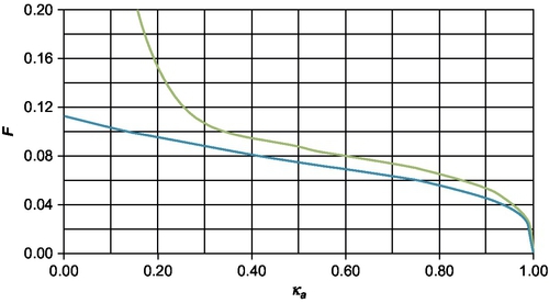
A failure-reducing behavior as a function of the κ_a is to be expected as this index approaches its maximum value. Figure 7.14 shows the behavior of the failure index F due to variation in the partial index of amplitude-complementarity.

Systems with π_Mm less than unity show failure slightly higher than those with π_Mm above unity. If a smaller battery bank is used, the curve is shifted up. The reverse is verified for bigger batteries. The shape of these lines is obviously related to the definition of the amplitude-complementarity index and must undergo changes with real data.

The use of idealized data brings out various aspects of the performance of hybrid hydroelectric-photovoltaic systems running on complementary energy resources. This procedure helps define the applicability of the system and supports the sizing of its components.

A better time-complementarity is associated to smaller failure indexes. A reservoir may artificially improve time-complementarity, having the effect of delaying the low hydro availability period. The value of the failure index may supply an initial value for the required water reservoir volume, and is strongly related to the conditions of the plant location.

A bigger contribution of hydroelectric origin leads to failure reduction, while an increased photovoltaic contribution implies a higher energy accumulation capacity. This result points to the applicability of hydroelectric-photovoltaic systems when hydro availability is insufficient to supply consumer demand.

A better amplitude-complementarity is associated to lower values of the failure index. A water reservoir may artificially improve amplitude-complementarity, transferring water from one semester to be used in the other, approaching the annual hydro availability distribution tending to the unity value for the index. But this, obviously, involves high costs.

The water reservoir design may aim at improving complementarity characteristics, causing imperfect natural complementarity to improve and to approach a situation leading to a better operation of the hybrid system.

Operation strategy and the design of the cheapest components should consider the investment objective of the reservoir, seeking the best possible use for the stored water.

All these comments are valid for other types of energy storage. This work considers the ways that are most obviously associated with hydropower plants and with photovoltaic modules.

7.8 Some Real Hybrid Systems with Partial Complementarity

It is interesting to compare the results of the previous section with results of real systems. In this section, some results of case studies are presented, for which feasibility studies were performed with Homer [Lambert et al., 2005; Lilienthal et al., 2004]. These case studies were originally seeking optimal combinations of the components of the systems to meet consumers. Here, issues related to complementarity are discussed. Three case studies will be reviewed.

Beluco et al. (2013a) sought an optimal solution for power generation during peak hours for a recycled paper factory in southern Brazil. The load is 328 kW of installed capacity, with daily consumption of 975 kWh. The study considered two possible alternatives for power generation during peak hours, both with diesel support and possible connection to the grid.

One alternative considered the restoration of an old plant with 240 kW. The other considered a plant to be undertaken with a power of 427 kW. The two alternatives considered installing PV modules on the roof of the factory building with an area of about 1 ha. The company already had three diesel generators, two with 150 kW and one with 30 kW.

For the first alternative, the index of complementarity in time is equal to 0.98, the complementary energy is equal to 0.82, and complementarity between amplitudes is 0.78. For the second alternative, the index of complementarity in time is equal to 0.92, the complementary energy is equal to 0.74, and complementarity between amplitudes is 0.89.

Observing the annual availabilities of the two resources, the high values of complementarity in time, 0.98 and 0.92, respectively, are evident. Figure 7.15 shows the water availability for the two alternatives, and Figure 7.16 shows the solar availability. Figure 7.17 shows the behavior of the system, obtained by simulations with Homer, for a period of one year.

This system does not use batteries, inserting excess energy in the grid and recovering energy from there when needed. This simulation was performed with low cost for diesel oil, and so the diesel generator set is fired over the hydroelectric plant at precisely the time of year with greater water availability. Building a reservoir, if possible, could allow the use of complementarity in favor of the system, possibly eliminating the need for diesel support.

Silva et al. (2012) studied the case of a middle-class family intending to install a PV-wind-diesel hybrid system that gives them independence from the grid. The study focuses on the costs to be achieved by the PV modules so that solutions can count on photovoltaics. The house is located in the city of Porto Alegre in southern Brazil, has a total area of about 160 square meters, and has a consumer load of 2.6 kW peak, with a daily consumption of 10 kWh. Water heating represents a load of 0.625 kW peak and a daily consumption of 15 kWh.

The system has a small wind turbine, a diesel gen set, PV modules, and the possibility of connection to the grid, plus a small battery bank. Figure 7.18 shows the solar and wind energy availability for this hybrid system, indicating null complementarity. Figure 7.19 shows the results provided by Homer to this system for a period of one year.

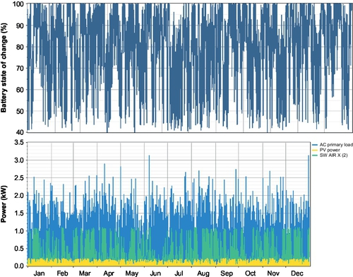
The comparison between solar and wind availability is always difficult because of the variability of wind. Periods of minimum availability of the two resources match in June. If there was complementarity, optimal combinations of components that include PV modules would be obtained with current pricing.

These results are different from the previous ones because climatological effects and a variable demand profile make it difficult to analyze the results. The lack of complementarity and the inconstancy of the winds lead to daily and constant use of the batteries. The power drawn by consumers has many variations, but due to the demand profile, it is not constant. This system does not fail.

7.9 Effects of Energy Storage

The simulations presented here consider only the energy storage in batteries. The study of hydro-PV hybrid systems opens the way for the possibility of accumulation of water in a reservoir. Several results show excess water in one semester and lack of energy in the other semester. A reservoir sized for one or two weeks of consumer demand can solve the problem.

This topic is still the subject of research projects, and the use of a reservoir in combination with batteries can be a complex problem of optimization of resources available for energy storage. The costs of a reservoir and environmental concerns should make its use impractical, but its consideration in studies of complementarity can shed new light on the analysis of its viability.

Just as an example, the system shown in Figure 7.8(d) was simulated again, now with a reservoir included in the system: a water reservoir with a capacity equivalent to 20 days of energy consumption. Its use was linked to low stored energy in the batteries and the imminent failure of the power supply to consumers.

Figure 7.20 shows the results of this simulation. The left graph was assembled the same as the previous ones, indicating the general state of charge of the two storage devices. The graph to the right details the SOC in medium gray line forming a more widespread spot, and the state of charge of the reservoir in dark gray. The main result is that faults are reduced to zero, as was to be expected!

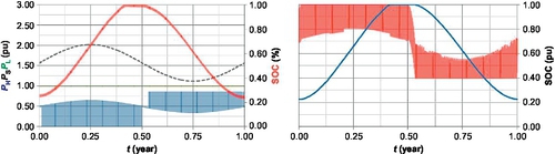
As the capacity of the reservoir is much larger than the capacity of the batteries, it is observed that the first is almost not influenced by the second. The reservoir is filled during the months of highest water availability and emptied when necessary. It is also observed that the hydroelectric plant always operates at full capacity in the second half.