15.3 The Pareto Frontier
The Pareto Frontier and Dominance
The Pareto frontier [2] is a set of architectures that form the “edge of the envelope,” colloquially speaking. Because we have two or more metrics represented in a tradespace, it is unlikely that any single architecture is uniquely “the best.” Rather, the Pareto frontier, also known as the Pareto front, showcases the architectures that are “good” and represent good tradeoffs between the metrics.
Consider, for example, the simple tradespace given in Figure 15.2, which contains three engines from Figure 15.1 (A, B, and C). Note that performance and cost are in tension: Low cost and high performance are good, but increasing performance generally requires increasing cost, as Figure 15.1 confirms.
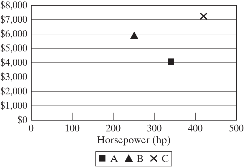
Figure 15.2 A simple tradespace with a few engines, using performance (hp) and cost as metrics.
The key concept for the Pareto front is dominance: The set of non-dominated architectures is called the Pareto frontier. An architecture A1 strongly dominates another A2 if A1 is better than A2 in all metrics. If A1 is at least as good as A2 in all metrics, and better than A2 in at least one metric, we say that A1 weakly dominates A2. If no architecture dominates an architecture A1, then A1 is said to be non-dominated.
In the simple example of Figure 15.2, engine B is objectively worse than A: Engine A can provide more power than B at lower cost. Engine B is dominated by engine A. Engines A and C are not dominated by any other engine; that is, they are non-dominated and on the Pareto frontier. Engine B is not on the Pareto frontier. There is no objective way of assessing, on the basis of this information, which of A and C is better; we need to include other information in order to refine our preferences.
The Pareto Frontier of a GNC System Example
To see what a Pareto front looks like in a more complex case, we will now introduce an example based on a guidance, navigation, and control (GNC) system. GNC systems are an essential component of autonomous vehicles—cars, aircraft, robots, and spacecraft. They measure the current state (position and attitude of the vehicle), compute the desired state, and create inputs to actuators to achieve the desired state. A key feature of such systems is extremely high reliability, which is often achieved by having multiple (and sometimes interconnected) paths from sensors to actuators.
We return to our observation from Chapter 14 that, in general, the screening metrics for a system are some combination of performance, cost, and developmental or operational risk. In the GNC case, we assume that all architectures give adequate performance, and we focus on mass and reliability. Mass is important for all vehicles because they need to carry their own weight, and mass has a significant impact on cost. Reliability is a key concern in system-critical autonomous systems, especially those where remote maintenance is very costly or impossible.
We further assume that we have three types of sensors available (A, B, C), with increasing mass and reliability (more reliable components are generally heavier); three types of computers (A, B, C), also with increasing order of mass and reliability; and three types of actuators (A, B, C). We have one generic type of connection, which we initially assume is massless and of perfect reliability. For this example, we can define the decisions as the number and type of sensors, of computers, and of actuators, each up to three. Initially there is no penalty for choosing different types of, say, actuators. Another architectural decision is the number and pattern of the connections, with the constraint that every component must be connected to at least one other component.
To be more concrete, an autonomous car could have three different sensors (sonar sensors to determine range to cars in front, a GPS receiver, and a cornering accelerometer), three computers, one of a different type (one FPGA and two microprocessors), and three similar actuators (an electric motor for the front wheels, a larger electric motor for the rear wheels, and a gas engine that can directly drive the front wheels).
Given the symmetry of the problem in the connections between sensors and computers, and between computers and actuators, we will look only at the sensor–computer part of the problem. Figure 15.3 shows some valid architectures.
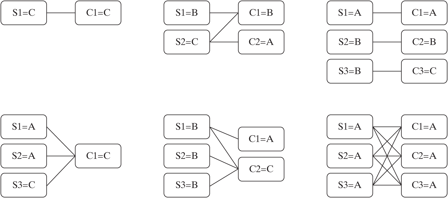
Figure 15.3 Pictorial representation of some valid architectures for the GNC problem. Architectures consist of a number of sensors of type A, B, or C, connected in a topology to a set of computers of type A, B, or C. Note the high level of abstraction at which we work, allows us to formulate a decision-making problem that captures the main trades of interest—in this case, mass versus reliability.
For each architecture, boxes represent sensors (S) and computers (C) of different types (A, B, C), and lines represent interconnections between them. Figure 15.4 shows the tradespace of mass versus reliability for the 20,509 valid architectures, with the Pareto frontier highlighted with a solid line.
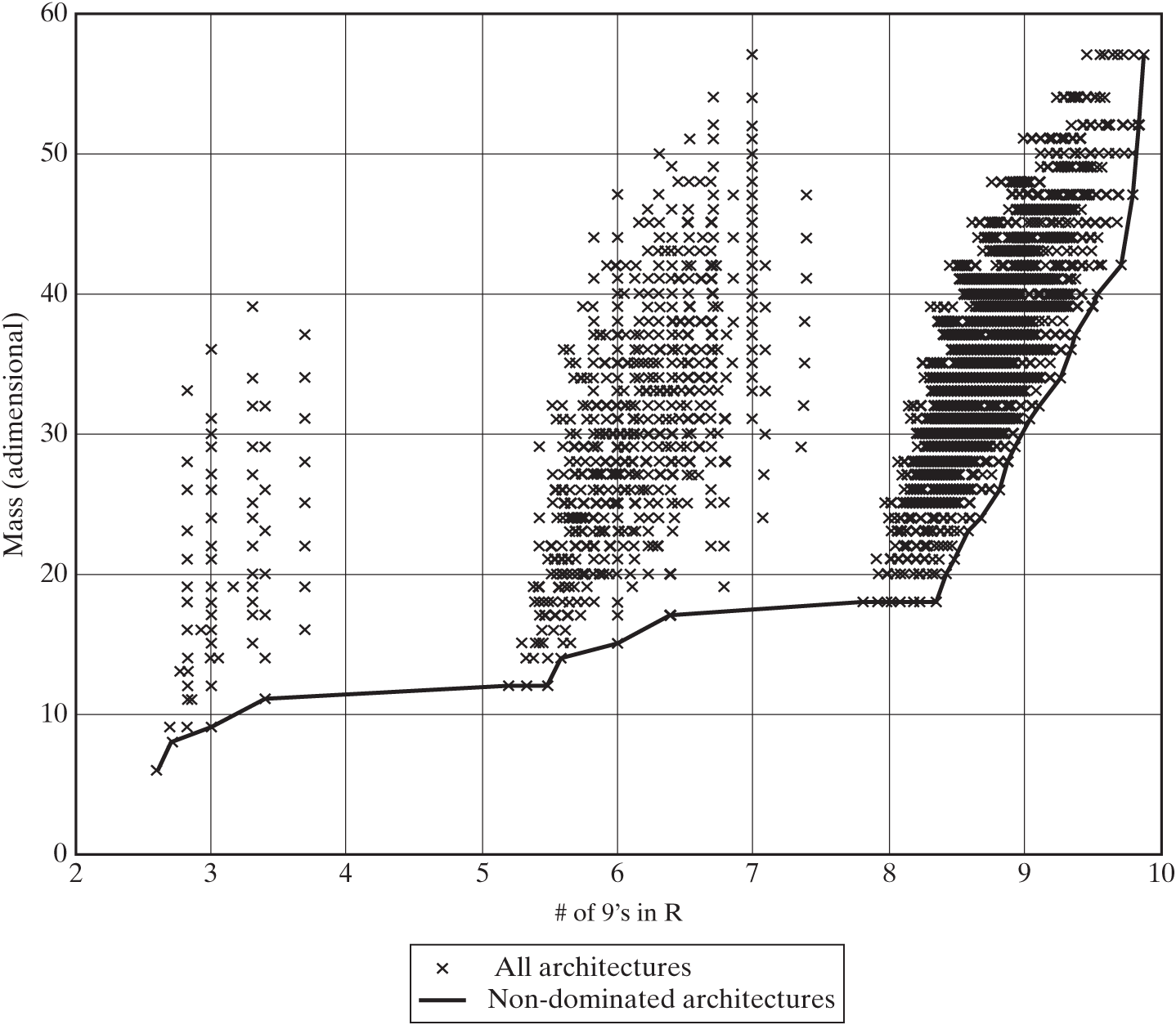
Figure 15.4 Mass–reliability tradespace for the GNC example, with the Pareto front highlighted. The number of nines (# of 9’s) in the reliability is shown instead of the reliability value (for example, 3 nines is equivalent to R = 0.999, and R = 0.993 is equivalent to 2.15 nines).
Let’s assume that we want to be in the region of the space with at least 0.99999999 (colloquially known as “8 nines”) of reliability. We can zoom in on that region of the tradespace, and see what some architectures on this region of the Pareto front look like. This is shown in Figure 15.5.
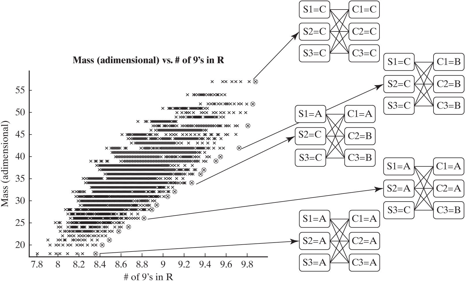
Figure 15.5 Zooming in on the high-reliability region of the mass–reliability tradespace. Some architectures on the Pareto frontier are pictorially illustrated.
Four architectures that lie on the Pareto frontier are represented on the righthand side of Figure 15.5. For example, the top-right architecture consists of three sensors of type C and three computers of type C, with all possible connections between them. This architecture achieves the highest reliability at the highest mass, as expected.
When analyzing a Pareto plot, our first instinct must be to look for the Utopia point, an imaginary point on the tradespace that would have the best possible scores in all metrics. In Figure 15.4 and Figure 15.5, the Utopia point is at the bottom right of the plot, ideally with maximum reliability and minimum mass. Non-dominated architectures typically lie on a convex curve off the Utopia point. Visually, we can quickly find the approximate Pareto frontier of a tradespace plot by moving from the Utopia point toward the opposite corner of the tradespace plot; the first points that we find—those that are closest to the Utopia point (engines A and C in Figure 15.2)—usually form the Pareto frontier. Note, however, that the numerical distance from an architecture to the Utopia point cannot be used to determine whether one architecture dominates another.*
Despite the density of architectures in the tradespace enumerated in Figure 15.5, the Pareto front is not smooth. Unless there is a simple underlying function governing the tradeoff (for instance, antenna diameter is a square root function of data rate in a communication system), it is rare for the Pareto front to be smooth. Irregularities are caused by discrete and categorical decisions and shifts between technologies. However, there is a shape to the front; it is roughly running up and right but “curving left,” indicating that gains in reliability require successively greater mass investment. This type of “knee in the curve” around 9.7 R’s is frequently interpreted as a balanced tradeoff in decisions.
The Fuzzy Pareto Frontier and Its Benefit
Dominated architectures are not necessarily poor choices. Some slightly dominated architectures may actually outperform non-dominated ones, judging on the basis of other metrics or constraints not shown in the plot, and this makes them excellent candidates for further study.
The concept of fuzzy Pareto frontier was introduced to capture a narrow swath of choices near the frontier. The fuzzy frontier can be an explicit acknowledgment of performance uncertainty, ambiguity in measurement, errors in the model, or the like. Moreover, architectures that are non-dominated in a few metrics (such as performance and cost) are sometimes the least robust in responding to variations in model assumptions. [3] When we are dealing with families of architectures, we sometimes find that one key member of the family is slightly off the frontier. The main idea is to relax the Pareto filter condition so that slightly dominated architectures that may subsequently be important are not discarded. A method for computing the fuzzy frontier is given in the next section. The fuzzy Pareto frontier represents our first cut at reducing the tradespace down to a manageable decision.
Mining Data on the Fuzzy Pareto Frontier
In Figure 15.5, all architectures on the frontier appear to be fully cross-strapped; that is, all sensors were connected to all computers. This suggests that fully cross-strapped architectures may be dominating the Pareto frontier. How can we perform this analysis in a systematic way?
Simply plotting the architectures with the same decision choice using the same color or marker is a simple way to view the results. For example, Figure 15.6 is a view of the same tradespace, where non-dominated cross-strapped architectures are highlighted using squares. The Pareto frontier is still shown by the solid line. It is apparent from Figure 15.6 that all architectures on the Pareto front are fully cross-strapped.
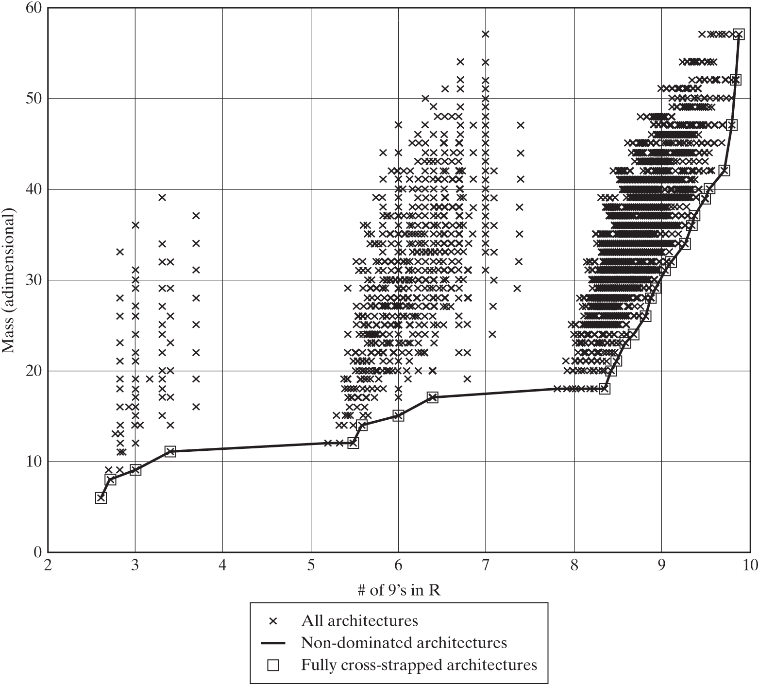
Figure 15.6 Tradespace for the GNC example, where all non-dominated architectures are shown to be fully cross-strapped.
When graphical methods are not conclusive, a simple quantitative method is to compute the relative frequency with which a certain architectural decision is set to a certain alternative inside and outside the (fuzzy) Pareto frontier. If the percentage of architectures with alternative is significantly higher inside the Pareto frontier than outside the Pareto frontier, this would suggest—though not prove—that there is a correlation between choice and the non-dominated architectures.
Table 15.2 shows statistics on the Pareto frontier of Figure 15.5. Three features are analyzed:
Table 15.2 | Percentage of architectures on the GNC Pareto front that share a common architectural feature (that is, a particular decision choice or combination of decision choices) and other, related statistics
| Architectural feature | % architectures with this feature in entire trade space | % architectures of the Pareto front that have this feature | % architectures with this feature that are on the Pareto front |
|---|---|---|---|
| Fully cross-strapped | 2% | 100% | 7% |
| Homogeneous (one type of sensors and computers) | 7% | 33% | 1% |
| Uses one or more sensors of type C | 59% | 56% | 0.1% |
Fully cross-strapped versus not fully cross-strapped.
Homogeneous (using a single type of sensor and a single type of computer) versus non-homogeneous.
Architectures that have one or more sensors of type A versus those that don’t.
Table 15.2 confirms that “fully cross-strapped” is a dominant architectural feature: Only 2% of the architectures enumerated in the tradespace are fully cross-strapped, and yet all non-dominated architectures are fully cross-strapped. Being fully cross-strapped appears to be a necessary condition for an architecture to lie on the Pareto front.
The case of homogeneous architectures is similar in that only 7% of architectures in the tradespace are homogeneous, but all of them lie on the Pareto front. However, this feature is not as dominant as the “fully but a disproportionately high percentage of non-dominated architectures are homogeneous” condition: Only 33% of the architectures on the Pareto front are homogeneous. In other words, homogeneity is not a necessary condition to lie on the Pareto front; there are ways to achieve non-dominance even for non-homogeneous architectures.
Conversely, 59% of the architectures in the tradespace use one or more sensors of type C, but about the same percentage (56%) of non-dominated architectures have this feature. This clearly suggests that having one or more sensors of type C is not a dominant feature.
Eliminating architectures that are not on the Pareto front is a means for down-selecting architectures, but it is not the sole method. Pareto dominance may not be useful for selecting architectures when the number of metrics increases. Indeed, in large-dimensional objective spaces, the number of non-dominated architectures is simply too high to be useful. Therefore, Pareto dominance needs to be seen as one filter used to discard poor (highly dominated) architectures, rather than as an algorithm sufficient by itself to obtain a manageable set of preferred architectures.
Pareto Frontier Mechanics
How do we compute the Pareto frontier in a general tradespace with thousands or millions of architectures and several metrics? If we generalize what we did in our trivial example of the engines in Figure 15.2, an algorithm for computing a Pareto front requires comparing each architecture to all other architectures in all metrics. Therefore, in a tradespace with N architectures and M metrics, the algorithm takes, in the worst case, ( comparisons to find the non-dominated set.
Sometimes, it can be interesting to compute Pareto fronts in a recursive fashion in order to sort architectures according to their Pareto ranking. This process is called non-dominated sorting. An architecture that is non-dominated has a Pareto ranking of 1. To find the architectures with Pareto ranking 2, we simply discard architectures with Pareto ranking 1 and compute the new Pareto frontier by following the same procedure. The architectures on the new Pareto front have a Pareto ranking of 2. We repeat this process recursively until all architectures have been assigned a Pareto ranking. This algorithm takes on the order of N times . Faster algorithms exist for non-dominated sorting that keep track of the dominance relationships, at the expense of memory usage. [4]
Pareto ranking can be used as a metric for architecture selection. For example, given the Pareto rankings of a set of architectures, it might be a good idea to discard architectures that have very bad Pareto rankings (in other words, those that are heavily dominated).
A straightforward implementation of a fuzzy Pareto filter is based on non-dominated sorting. For instance, a fuzzy Pareto frontier may be formed with architectures that have a Pareto rank less than or equal to 3. This implementation of fuzzy Pareto fronts is mathematically elegant, but it does not take into account the distance in the objective space between architectures with different Pareto rankings. As a result, one might discard an architecture that is in a region of very high density of architectures, and is very close to the first Pareto frontier, on the basis of a high (that is, poor) Pareto rank. To address this problem, an alternative implementation of fuzzy Pareto fronts computes the true Pareto front and then discards all points that have a distance to the Pareto front greater than some threshold (such as 10% Euclidean distance in a fully normalized objective space).