14.5 Basic Decision Support Tools
We have already seen, in Parts 2 and 3, examples of tools that are useful in some of the four layers of decision support. For example, we used Object Process Methodology (OPM) to represent not only system architectures but also specific decision-making problems, such as function or form specialization (see, for example, Figure 7.2). We introduced morphological matrices as a means to represent simple decision-making problems, such as concept selection (see, for example, Table 7.10). We also used Design Structure Matrices in Part 2, mostly to represent the interfaces between entities of a system.You are already familiar with tools that are useful in some of the four layers of decision support, such as Object Process Methodology (OPM), morphological matrices, and Design Structure Matrices (DMSs). In Part 4, we focus on the other aspects of decision support: structuring, simulating, and viewing.
We start this section by revisiting morphological matrices and DSMs, showing that these tools provide limited support to structuring, and no support to simulation and viewing. Then we introduce decision trees as a widely used decision support tool for decision making under uncertainty, providing some support to the structuring and simulating layers. (Other widely used decision support tools, such as Markov Decision Processes, are not described in this section because they are seldom used for system architecture purposes.)
Morphological Matrix
The morphological matrix was introduced in Chapter 7 as a way to represent and organize decisions in a tabular format. The morphological matrix was first defined by Zwicky as a part of a method for studying the “total space of configurations” (morphologies) of a system. [22] Since then, the use of morphological matrices as a decision support tool has grown. [23] Figure 14.1 includes the morphological table for the Apollo example.
A morphological matrix lists the decisions and associated alternatives, as shown in Figure 14.1. An architecture of the system is chosen by selecting one alternative (labeled “alt”) from the row of alternatives listed to the right of each decision. Note that alternatives for different decisions do not have to come from the same column. For example, a configuration of the Apollo system could be: number of EOR = no (alt A), LOR = yes (alt B), command module crew = 2 (alt A), lunar module crew = 2 (alt C). An example of an expanded or more explicit form of the morphological matrix was given in Table 7.10.
In terms of decision support, the morphological matrix is a useful, straightforward method for representing decisions and alternatives. It is easy to construct and simple to understand. However, a morphological matrix does not represent metrics or constraints between decisions. Thus it does not provide tools for structuring a decision problem, simulating the outcome of decisions, or viewing the results.
Design Structure Matrix
As introduced in Chapter 4, a Design Structure Matrix is actually a form of decision support. The term Design Structure Matrix (DSM) was introduced in 1981 by Steward. [24] DSMs are now widely used in system architecture, product design, organizational design, and project management.
A DSM is a square matrix that represents the entities in a set and their bilateral relationships (see Table 4.4). These entities can be the parts of a product, the main functions of a system, or the people in a team, as demonstrated in the different examples throughout Part 2.
When a DSM is used to study the interconnections between decisions, each row and column corresponds to one of the N decisions, and an entry in the matrix indicates the connections, if any, that exist between the two decisions. The connections could be logical constraints or “reasonableness” constraints, or they could be connections through metrics.
Table 14.3 | DSM representing the interconnection of decisions by logical constraints for the Apollo case
| 1 | 2 | 3 | 4 | 5 | 6 | 7 | 8 | 9 | ||
| EOR | 1 | a | ||||||||
| earthLaunch | 2 | a | ||||||||
| LOR | 3 | b | c | e | f | |||||
| moonArrival | 4 | b | ||||||||
| moonDeparture | 5 | c | ||||||||
| cmCrew | 6 | d | ||||||||
| lmCrew | 7 | e | d | |||||||
| smFuel | 8 | |||||||||
| imFuel | 9 | f |
For example, in Table 14.3, the letter a at the intersection between “EOR” and “earthLaunch” indicates that there is a connection between these two decisions as the result of the constraint labeled “a” in Table 14.1. Likewise, the letters b through f indicate the other five constraints. A blank entry in the intersection indicates that there is no direct connection between these decisions imposed by the constraints.
A connection could mean that a metric depends on those two variables. For example, Table 14.4 shows the connection between the decisions given by the IMLEO metric. The entries in the matrix may have different letters, numbers, symbols, or colors to indicate different types of connections.
Table 14.4 | DSM representing the interconnection of decisions by the IMLEO metric in the Apollo case
| 1 | 2 | 3 | 4 | 5 | 6 | 7 | 8 | 9 | ||
| EOR | 1 | |||||||||
| earthLaunch | 2 | |||||||||
| LOR | 3 | I | I | I | I | |||||
| moonArrival | 4 | |||||||||
| moonDeparture | 5 | |||||||||
| cmCrew | 6 | I | I | I | I | |||||
| lmCrew | 7 | I | I | I | ||||||
| smFuel | 8 | I | I | I | ||||||
| imFuel | 9 | I | I | I |
In Table 14.5, the DSM of Table 14.3 has been partitioned and sorted so as to minimize interactions across blocks of decisions when possible. These blocks represent sets of decisions that should be made approximately simultaneously, because they have couplings with each other (for example, LOR with Lunar Module crew, Service Module crew, Service Module fuel, Lunar Module fuel). A partitioning procedure and example are given in Steward’s papers. More generally, clustering algorithms can be used for partitioning (see Appendix B).
Table 14.5 | Sorted DSM of the interconnections of decisions by logical constraints for the Apollo case
| 1 | 2 | 3 | 4 | 5 | 6 | 7 | 9 | 8 | ||
| EOR | 1 | a | ||||||||
| earthLaunch | 2 | a | ||||||||
| LOR | 3 | b | c | e | f | |||||
| moonArrival | 4 | b | ||||||||
| moonDeparture | 5 | c | ||||||||
| cmCrew | 6 | d | ||||||||
| lmCrew | 7 | e | d | |||||||
| imFuel | 9 | f | ||||||||
| smFuel | 8 |
A DSM provides information in the representing layer and the structuring layer of decision support. It represents the decisions (but not their alternatives) and their interconnections. In combination with partitioning or clustering algorithms, a DSM can be sorted to show which sets of decisions are tightly coupled and which sets are less tightly coupled or not coupled. This information informs both system decomposition and the timing of architectural decisions, if the order of the decisions in the matrix is taken to represent the sequence in which they are made. [25]
Decision Trees
A decision tree is a well-known way to represent sequential, connected decisions. A decision tree can have three types of nodes: decision nodes, chance nodes, and leaf nodes. Decision nodes represent decisions, which are controllable by the decision maker and have a finite number of possible assignments represented by branches in the tree from that node. Chance nodes represent chance variables, which are not controllable by the decision maker and also have a finite number of possible assignments, which are also represented by branches. The endpoints, or “leaf” nodes, in the decision tree represent a complete assignment of all chance variables and decisions.
When these decisions are architectural decisions, a path through the decision tree essentially defines an architecture. Thus, decision trees without chance nodes can be used to represent different architectures. Figure 14.4 shows a decision tree for the Apollo example concerning the five decisions related to the mission-mode. All nodes in this chart are decision nodes except for the final node in each branch, which is a leaf node. The first three of the constraints of Table 14.1 have also been implicitly included in the tree; for example, if earthLaunch = yes, there is no option of EOR = yes. This branch has been “pruned” from the tree by applying the logical constraint.
Note that this decision tree representation explicitly enumerates all the combinations of options (that is, all architectures), whereas the morphological matrix enumerated architectures only implicitly, by showing the alternatives for each decision. A limitation of decision trees is immediately visible in Figure 14.4: The size of a decision tree grows rapidly with the number of decisions and options, which results in huge trees, even for modest numbers of decisions.
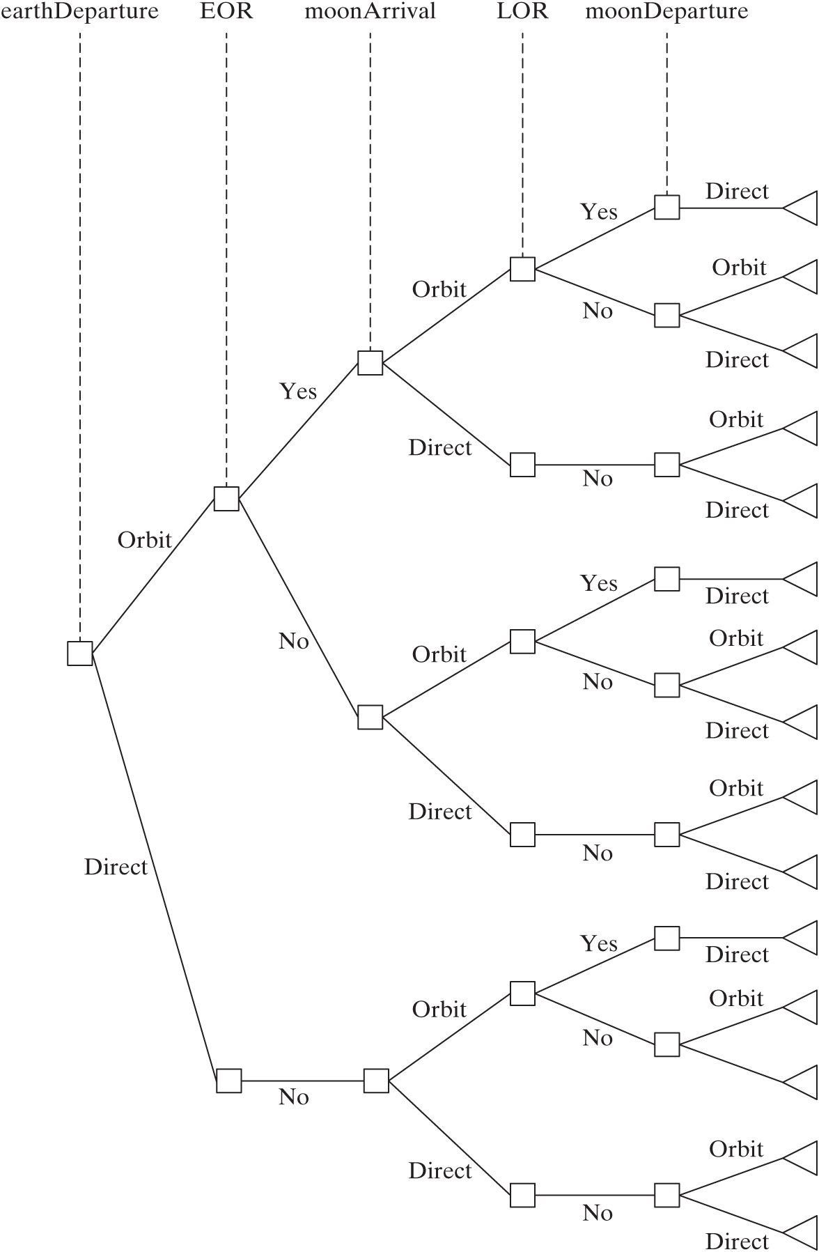
Figure 14.4 Simple decision tree with only decision nodes and leaf nodes (no chance nodes) for the Apollo mission-mode decisions.
In addition to representing architectures, decision trees can be used for evaluating architectures and selecting the best ones. This requires computing the metrics for each architecture. Sometimes, it is possible to compute a metric incrementally while following a path in the tree. For example, the probability-of-success metric in the Apollo example can be computed in this way, because the contribution of each decision to the overall probability of success is given by Table 14.2, and the metric is constructed by multiplying the individual contributions together.
In most cases however, there is coupling between decisions and metrics that is not additive or multiplicative, such as in the case of the IMLEO metric, a highly nonlinear function of the decision alternatives. In these cases, the metric for every leaf node (such as IMLEO) is usually computed after all the decision alternatives have been chosen. This approach may be impractical in cases where the number of architectures is very large, as we will see in Chapter 16.
The leaves or architectures represented on decision trees are usually evaluated using a single metric. In such cases, it is customary to combine all relevant metrics (such as IMLEO and probability of success ) into a single metric representing the utility of an architecture for stakeholders [such as u = au (IMLEO) + (1 − a) u(p)]. The weight a and the individual utility functions u (IMLEOand u(p can be determined by means of multi-attribute utility theory. [26]
In decision trees that don’t have chance nodes, choosing the best architecture is straightforward. It is more complicated in the presence of chance nodes, because leaf nodes no longer represent architectures but, rather, combinations of architectures and scenarios. It is thus necessary to choose the architecture that has the highest expected utility by working backwards from the leaf nodes. Let’s illustrate that with an example.
Assume that, instead of having a single value for the risk factor of each decision in Table 14.2, we had two values: an optimistic one and a pessimistic one. What is the best architecture given this uncertainty? Figure 14.5 shows the addition of the chance nodes corresponding to the last decision in the tree for the Apollo case (only a very small part of the tree is actually shown). Note that the actual tree has effectively doubled in size just through the addition of chance nodes corresponding to the moonDeparture decision. We compute the risk metric for all the new leaf nodes by traversing the tree from start to finish and multiplying all the risk factors together (the results are the Ri values in Figure 14.5). At this point, we can’t simply choose the leaf node with the lowest risk, because it does not represent an architecture; it represents an architecture for a given scenario—that is, a value of the risk factors. Instead, we need to assign probabilities to the branches of the chance nodes (such as 50%-50% everywhere), and compute the expected value of the risk metric at each chance node. Then, it makes sense to choose the Moon departure option with the lowest risk at each decision node. If we add chance nodes to all the other decisions, we can follow the same two steps. First, we compute the expected risk factor at each chance node, and then we pick the option with the best risk metric. We perform these steps for the LOR decision, then the moonArrival decision, and so forth, until all decisions have been made. This process yields the architecture that has best performance on average across all scenarios. This architecture is given by the combination of all the optimal decisions.
In short, the best architecture in a decision tree can be found by applying these two steps (expectation for chance nodes and maximization/minimization for decision nodes), starting from the leaf nodes and going backwards through the tree. [27]
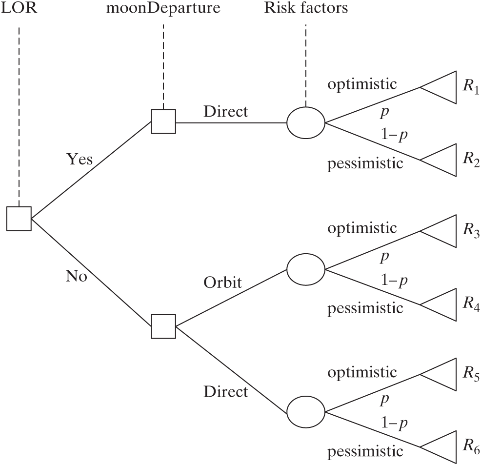
Figure 14.5 Fragment of the Apollo decision tree, including a chance node for the risk factors. In this tree, decision nodes are squares, chance nodes are circles, and leaf nodes are triangles. Ri are the values of the risk metrics for each architecture fragment, and p is the probability of being in an optimistic scenario for each individual decision. (Note that these probabilities could in general be different for different chance nodes.)
Even though they are commonly used as general decision support tools, decision trees have several limitations that make them impractical to use in large system architecture problems. First, they require pre-computation of a payoff matrix containing the utilities of all the different options for each decision for all possible scenarios, which may be impractical for many problems. More generally, their size grows exponentially with the number of nodes in the problem.
Second, the method assumes that the payoffs and probabilities for a given decision are independent from the rest of the decisions, which is often unrealistic. For example, consider that instead of modeling the uncertainty in the risk factors, we wish to model the uncertainty in the ratio between propellant mass and structure mass for any of the vehicles used in the architecture. This is a very important parameter of the model, because it can drive the IMLEO metric. However, this parameter does not directly affect any of the decisions the way the risk factor did. It affects the IMLEO metric through a complex mathematical relationship based on the mission-mode decisions. This ratio is thus a “hidden” uncontrollable variable that affects multiple decisions. Modeling this in a decision tree is very difficult, or else it requires collapsing all the mission-mode decisions into a single decision with 15 options (the number of leaf nodes in Figure 14.4).
In summary, decision trees provide a representation of the decision and can represent some kinds of structure, but they are of limited use in simulation.*