
Crude Oil
Abstract
Oil has been the number one source of energy in the world since the middle of the twentieth century. The world is very dependent on petroleum for transportation fuels, petrochemicals and asphalt. But ever increasing demand has caused the price of oil to spike in recent years, and only the world economic crisis has been able to temper demand and bring the price down to more reasonable levels. However, the demand and price are likely to shoot up again when the economy recovers. At the same time, the peak oil theory of M. King Hubbert predicts that world oil production is likely to peak soon. This prediction raises questions about what source of energy will come to the fore when oil is not able to keep up.
Oil is the number one source of energy in the world and has held this place since the middle of the twentieth century. The world is very dependent on oil for transportation fuels, petrochemicals and asphalt. The ever increasing demand has caused the price to spike in recent years and only the world economic crisis has been able to temper demand and bring the price down to more reasonable levels. Once the economy recovers, the demand and price are likely to shoot up again. At the same time, the peak oil theory of King Hubbert predicts that world oil production is likely to peak soon, and this will place even more upward pressure on the price of oil. This raises two questions: when is oil production likely to peak and what source of energy will come to the forefront if and when oil is not able to keep up?
The theories of Hubbert have garnered a lot of credibility after his successful prediction of the rise and fall of oil production in the United States. His prediction, however, that world oil production would peak in 2000 and fall rapidly after that has not proven true. Eleven years later, the world oil production continues to rise according to the demands of the world economy. Despite evidence to the contrary, Hubbert’s theories still have a lot of support and many people still expect that oil production is about to peak and will fall rapidly in the immediate future. They then expect that the world will be starved of energy and resource wars will follow that will plunge the world into a bitter struggle for control of the remaining resources that are rapidly depleting. Oil is a finite resource, and there is no denying the fact that at some point world oil production will peak and at some point in the distant future we will run out of it altogether. In this chapter, you will see that the world still has plenty of oil and that, if and when it does eventually peak, it will not decline as rapidly as Hubbert predicts.
Probably the leading exponent of Hubbert’s theories is Ken Deffeyes, a geologist who worked at the Shell Research Labs in the early 1960s as a colleague and protégé of Hubbert. Deffeyes has published three books that espouse his theories: Hubbert’s Peak: The Impending World Oil Shortage (Deffeyes, 2001); Beyond Oil: The View from Hubbert’s Peak (Deffeyes, 2005); and, When Oil Peaked (Deffeyes, 2010). After his early work with Hubbert, Deffeyes became a Professor of Geology, first at the University of Minnesota and then in 1967 at Princeton University. His first book (Hubbert’s Peak) forecast in 2001 that the oil shortage was about to start and forecast dire consequences for the world economy. His actual projection for the peak at that time was August 2004. His second book (Beyond Oil) slightly revised the forecast for the world oil production peak to occur in late 2005. In the preface to the paperback edition (written in 2006), he nominated December 16, 2005 as the actual date that world oil production peaked. In his third book (When Oil Peaked), he ignored the fact that the world oil production was still rising and continued to insist that production peaked in 2005. He pointed to the rapid increase in the oil price over the last six years and, in the preface to the 2008 edition of Hubbert’s Peak, he triumphantly says, “I told you so.”
Another popular book that espoused the sentiment behind Hubbert’s “peak oil theory” is Matthew Simmons’ Twilight in the Desert, also published in 2005 (Simmons, 2005). In this book, Simmons argues that the oil production of Saudi Arabia—the world’s largest oil exporter—has peaked and will soon begin to decline rapidly. He further predicted that this would precipitate a rapid decline in world oil supply, causing the price of oil to shoot up. In separate predictions, he made bets with people that the price of oil through the entire year of 2010 would average over $200/barrel. This bet was looking pretty safe when prices jumped up to $140/barrel in the middle of 2008, fueled by a robust world economy. Under the influence of the financial crisis of late 2008, however, prices plunged again and in 2010 the price averaged about $80/barrel. Simmons, an investment banker, made his predictions after being given access to the Society of Petroleum Engineers database of technical articles. He researched all of the articles that had come from Saudi Aramco (the national oil company of Saudi Arabia) and came to the conclusion that Saudi’s main oil fields were depleting rapidly and would soon begin to decline in production. Saudi Aramco, of course, denied his claims and asserted that Saudi Arabia had plenty of oil and the capacity to meet world demand for the foreseeable future. In fact, in May 2011 an influential Saudi Prince—Al-Waleed bin Talal—said that he wanted oil prices to drop so that the United States and Europe did not accelerate efforts to wean themselves off his country's supply. If Saudi Arabia was in fact facing their “twilight in the desert,” they would not be trying to keep the rest of the world addicted to oil because they would not be able to maintain the supply. Six years after the publication of Simmons’ book, world oil production continues to increase. Incidentally, Simmons also made a number of public statements about the Deepwater Horizon disaster in the Gulf of Mexico in 2010 that also proved to be untrue. For instance, in late April 2010 he predicted that BP would not be able to cap the well and would have to declare bankruptcy by July 2010. Simmons died of accidental drowning in early August 2010.
Another purveyor of the doom and gloom scenarios is Michael Klare, who has published a series of books on the issues including: Resource War: The New Landscape of Global Conflict (2001), Blood and Oil: The Dangers and Consequences of America’s Growing Dependency on Imported Petroleum (2005) and Rising Powers, Shrinking Planet (Klare, 2008). Klare—a journalist who writes for The Nation, Harper’s, Foreign Affairs and The Los Angeles Times—forecasts a bleak future “… of surprising new alliances and explosive danger.” His concern is not just for the shortage of oil and natural gas, but also for uranium, coal, copper and several other key resources.
There are many such books and articles, too numerous to review here, that follow a similar theme—the world is about to peak in oil production and, on the other side of the peak, as we slide down the back side of Hubbert’s curve, we will experience severe economic dislocation and terrible conflicts. What does this Peak Oil Theory really refer to and does it have any basis in truth?
U.S. World Oil Production and the Peak Oil Theory
The idea of a “Peak Oil Theory” grew out of a 1956 paper published by Marion King Hubbert, who was a geologist/geophysicist who worked at the Shell Research Lab in Houston, Texas. Hubbert used his middle given name and thus was universally known amongst his colleagues as King Hubbert, which euphemistically reflected the high regard that his colleagues held for his intellectual abilities. He was born in San Saba, Texas, in 1903 and attended the University of Chicago, where he received his B.S. in 1926, his MS in 1928, and his PhD in 1937, studying geology and geophysics. He then taught geology at Columbia University in New York City for seven years. In 1943, he joined Shell Oil Company, working at their Shell Research Lab in Houston. Even before joining Shell, he had a consuming interest in the finite limits to national and world oil production. He examined the data for many years before publishing his landmark paper in 1956 in which he proposed that any finite resource—oil, gas, coal or uranium—follows a bell-shaped curve in its production history. At some point, it reaches a peak and begins to decline and the decline in production will mirror the rise in production on the way up. The peak production rate and the timing of the peak production depend on the total reserves that exist and are to be discovered in the future. Given that the bell-shaped curve is a mirror image of itself, when half of the world’s reserves are produced, the production rate will begin to decline from that point. Hubbert turned to two of his colleagues, Wallace Pratt and Lewis Weeks (eminent geologists of their time both of whom worked for subsidiaries of ExxonMobil), to give him estimates for the ultimate recovery of oil and gas in the world and in the United States in particular. He used these estimates to project the forecasts that he published. Determining the ultimate reserves that are to be discovered and produced in the future was somewhat of a guessing game that made Hubbert uncomfortable. This led him to realize that if he had the right model he did not need to guess; the production data itself could be fitted to the model to determine what the ultimate reserves would be. From this model, he worked out some very elegant mathematical methods for forecasting the ultimate reserves. These reserve methods depended on the model he assumed for production and the exact equations for the bell-shaped curve, but this technique removed some of the uncertainty about the ultimate reserves.
After retiring from Shell in 1964, he became a senior research scientist for the United States Geological Survey until his second retirement in 1976. He also held positions as an adjunct professor of geology and geophysics at Stanford University from 1963 to 1968 and at UC Berkeley from 1973 to 1976. While working for the United States Geological Survey, he produced an update to his forecast for the world oil production in 1969.
Three of Hubbert’s bell-shaped curves that he presented are reproduced as Figures 5.1, 5.3 and 5.4. Figure 5.1 (which is figure 21 from Hubbert’s 1956 paper) shows his forecast for oil production in the United States. He used two estimates of the ultimate oil reserves (150 billion and 200 billion barrels). One of these was from Wallace Pratt and the other was the estimate from Lewis Weeks. Using the higher estimate, he forecast that U.S. oil production would peak in 1970 at a production rate of 3 billion barrels per year (8.2 million b/d). Figure 5.2 shows the actual oil rate in the United States on a monthly basis. The U.S. oil rate did actually peak in November 1970 at 10 million b/d and in 1970 the United States actually produced 3.5 billion barrels. Hubbert’s prediction was remarkably successful and this gave a lot of credibility to his methodology of what has now come to be known as Peak Oil Theory, or “Hubbert’s Peak.”

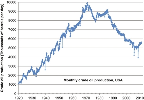
Two deviations on the monthly oil plot in Figure 5.2 deserve some explanation. After peaking in November 1970, U.S. oil production declined for six years in the manner predicted by Hubbert. From January 1977 to February 1986, the oil production rose again forming a secondary peak in that month at 9.14 million b/d. This deviation and secondary peak was due to the discovery and production of oil in the Prudhoe Bay and Kuparuk oil fields on the north slope of Alaska. Hubbert might argue that he did not take this area into consideration and that, excluding the Alaska oil production, the U.S. oil production from 1970 did decline in the manner that he predicted. The other deviation on the plot is the incline that has been occurring since late 2008 until the present time. This is due to oil production that is ramping up in the deep water of the Gulf of Mexico and the unconventional oil that is coming from the Bakken oil play in North Dakota. If allowed to continue, these oil sources are likely to cause U.S. oil production to keep increasing to form a tertiary peak sometime after 2020. Once again, Hubbert might argue that he was talking about conventional onshore oil and he did not take these unconventional plays into consideration. Despite these two deviations, Hubbert’s predictions for U.S. oil production proved to be remarkably accurate.
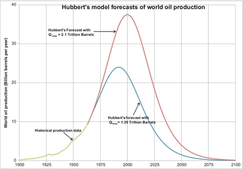
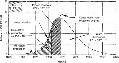
When Hubbert turned his attention to the forecast of world oil production, he produced the estimate shown in Figure 5.3 (his figure 20). This was based on ultimate oil reserves of 1.25 trillion barrels. His forecast showed a peak production of 12.5 billion barrels per year (34.25 million b/d), and it occurred in the year 2000. Later in his 1969 paper, he revised his numbers to show two estimates of ultimate recovery: 1.35 trillion barrels and 2.1 trillion barrels. The more optimistic 2.1 trillion barrel estimate again peaked in the year 2000 at 37.5 billion barrels per year (103 million b/d).
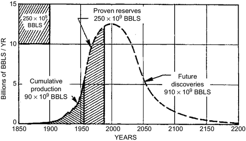
It is obvious that Hubbert’s forecasts depend on knowing how much oil can be discovered and produced in the world. Critics of his method say that this number is only a guess. How can you know how much oil is going to be eventually discovered in the world? Supporters point out that the timing of the peak is not sensitive to the actual number assumed for the ultimate recovery. Indeed, if you examine Figures 5.3 and 5.4 where three numbers are assumed for the ultimate recovery ranging from 1.25 trillion to 2.1 trillion barrels, the peak still occurs around the year 2000. Hubbert himself tackled this uncertainty and, borrowing from the mathematics of biological population growth and decay, he devised a mathematical method for forecasting the number for ultimate oil recovery. This mathematical method is shown in more detail in Appendix B. There you will see that Deffeyes predicts the ultimate world oil recovery will be 2 trillion barrels and that the peak oil production had already occurred in 2005.
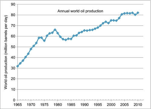
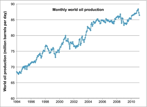
World oil production did not peak in 2000 or 2005. Figure 5.5 shows annual world oil production from 1965 to 2010, and at that time the production was still increasing. Figure 5.6 shows the world oil production on a monthly basis from the beginning of 1994 to early 2011, and though there are occasional declines, the overall trend on both plots is upwards and there is no evidence that a peak has occurred or will occur. The occasional dips in production that have occurred in the past 45 years are due to decreases in demand rather than decreases in supply. This does not stop the pundits from declaring that world oil production has peaked every time the production decreases from one year to the next or even from one month to the next. Figure 5.5 and Figure 5.6 use data from two different sources. The data for Figure 5.5 comes from the BP Annual Statistical Review, while the data for Figure 5.6 comes from the U.S. Energy Information Agency (EIA). Any discrepancies that are perceived between the two plots are due to the different data sources. What is important is that both plots show a consistent upward trend in world oil production. A secondary peak did occur in 1979 and, from 1979 to 1983, production did decrease. This was due to a steep increase in the world oil price in the 1970s, which resulted in decreased demand in the early 1980s as people reduced their use of transportation fuels. From 1983 to the present day, there has been a steady increase in oil demand which has been matched by supply. The world economic crisis that was precipitated in the middle of 2008 also tempered demand, causing a decrease in production in late 2008. From January 2009 to January 2011, there was a persistent increase in production. The uprising in Libya and other countries in the Middle East in early 2011, which is being called the “2011 Arab Spring,” has once again caused a new round of price increases and a resulting decrease in oil demand; however, this too is expected to be temporary. Using Hubbert’s model and the latest production data, you will see demonstrated in Appendix B that the peak in world oil production will not occur until at least 2018, and probably will be later than that.
So what is wrong with the Hubbert model and the analysis of his supporters that has caused their predictions about the timing of peak oil to be off? The Hubbert model is essentially correct under a constant price and constant technology scenario; however, when the oil price increases, the value of the ultimate recoverable oil (Qmax in Hubbert’s model discussed in Appendix B) also increases as more oil becomes economic to produce. In accordance with the cultural theories of Lesley White, discussed in Chapter 1, technology also has an impact.
From time to time, technology breakthroughs bring more oil reserves into production even under a constant price scenario. Additionally, when the price of oil increases, there is an incentive to develop new technologies which also increases the oil supply. Price increases and technology breakthroughs seem to unlock large volumes of oil that were previously not economic to produce. In the past 20 years, large reserves in the Canadian oil sands (a.k.a. tar sands, bitumen, ultra-heavy oil) have come on stream. New fracture stimulation and horizontal drilling technologies have also unlocked large reserves of tight oil, tight gas and shale gas. The Canadian oil sands in Alberta have currently booked reserves of 170 billion barrels, and the possible reserves reach as high as 1 trillion barrels. Compare that to the 1.3 trillion barrels of oil that have been produced in the world up until the present time and the 1 trillion barrels of conventional oil that Deffeyes said were left to be produced in 2005. Hundreds of billions of barrels of oil in the Bakken formation in North Dakota, Montana, Manitoba and Saskatchewan are also being unlocked with horizontal wells and multizone fracture stimulations. The success in the Bakken is also opening up more formations to successful production such as: the Eagle Ford in Texas; the Granite Wash in Oklahoma and the Texas Panhandle; the Niobrara in Colorado and Wyoming; the Monterey in California; the Utica formation in Eastern Ohio; and, the Shublik formation on the North Slope of Alaska. Vast quantities of oil have also been discovered in the deep waters of the Gulf of Mexico and in the Santos offshore basin in Brazil. As these technologies are developed, they will be applied to many other areas around the world.
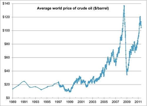
Figure 5.7 shows the average price of crude oil in the world since 1989 as determined by the EIA. The price increases of 2007-2008 and 2011 have accelerated the deployment of these new technologies as well as the economic development of other marginal reserves. From 1986 to 2005, the price of oil remained relatively constant at around $20/barrel, but the loud voices of the peak oil theorists in the twenty-first century probably caused the market to start anticipating supply shortages. This, and the political upheavals in the Middle East in 2011, has driven up the price of oil. At the same time, they have driven up the value of the world’s ultimate oil reserves, Qmax, and pushed out the timing of the peak production, tpeak. These developments not only affect Qmax and tpeak but will also affect the decline in production on the back side of the Hubbert curve. Oil will not be sliding down the other side of the curve in the manner that the Hubbert model forecasts or that the theorists expect. To illustrate this point, it is necessary to examine the U.S. natural gas production curves, which will be touched on in the next section of this chapter and examined in more detail in the following chapter. The history of the U.S. natural gas production has considerable relevance to the trends in world oil supply.
At this point, you might also ask why the Hubbert model worked so well in the prediction of the U.S. oil supply but did not seem to be working, and will not continue to work, for predicting the peak and decline in world oil supply. The answer is simple: the oil market is a world market and the U.S. oil production peaked and declined amidst a relatively constant world oil price. Even though the U.S. supply was decreasing, the world supply of oil was stable and the price remained relatively constant from 1986 to 2005. The Hubbert model works as long as the oil price and technology of extraction remains stable. The world price is now ramping upwards and this will profoundly change the dynamics of the Hubbert model.
Ken Deffeyes is fond of saying that, “The economists all think that if you show up at the cashier's cage with enough currency, God will put more oil in the ground.” God did not put any more oil in the ground, but between 2004 and 2010, the price of oil increased from $20/barrel to $100/barrel. This caused the tight oil in the Bakken and Eagle Ford formations, the heavy oil sands in Canada and the deepwater oil in the Gulf of Mexico and the Santos Basin to become economic to find and produce. In fact, another half trillion barrels of oil became economic to produce. In Appendix B, it is shown that if the monthly data published by the EIA and shown plotted in Figure 5.6 is used in the Hubbert model, an even more startling revelation emerges. When this data is extrapolated as shown in Appendix B, the predicted ultimate oil recovery, Qmax, is 3.055 trillion barrels. Of this 3 trillion barrels 1.3 trillion barrels has already been produced, leaving about 1.7 trillion barrels still to be found and produced. The current listed world-oil proved reserves according to the EIA is 1.3 trillion barrels, meaning that there are only 400 billion barrels still to be found. Remember, these numbers are a function of oil price and are likely to be conservative. Given that the data used for that extrapolation is probably the most reliable available data, this estimate is probably the most reliable estimate using current economics. It would seem that more oil is appearing all the time and this is due to economics. If and when the price of oil goes up again and stays up, these numbers will increase again.
The Hubbert model and the latest data give a peak oil date of October 23, 2018. Note that I am not saying that the world oil production will peak in October 2018. I am saying that using the Hubbert model and the latest and most accurate monthly world-oil production data the current projection for the peak oil rate is October 23, 2018. If the price of oil remained constant for the next seven years and there were no big technological breakthroughs during this time, this may prove to be an approximately accurate forecast. I don’t expect that this will be the case and so this date will probably move again.
The U.S. Gas Supply Analogy to World Oil Production
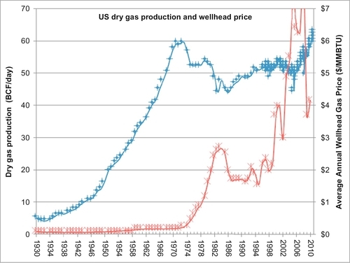
The U.S. gas supply trends have a lot of relevance to world oil supply behavior. In his 1956 paper, Hubbert made a forecast of U.S. natural gas production, which is reproduced in Figure 5.8 (his figure 22). This showed the nation’s gas production also peaking in the early 1970s (around1972) at about 14 trillion cubic feet per year (38 billion cubic feet per day), with an ultimate cumulative production (Qmax) of 850 trillion cubic feet. His figure also showed a line for the projected gas consumption rate which continues to increase after the nation’s gas production peaks and starts to decline. This was a projection using data supplied by Wallace Pratt. Figure 5.9 shows the actual U.S. dry gas production. The units of production on this plot are a billion cubic feet of gas per day, abbreviated as BCF/day. The data shows that the U.S. peaked in 1973 (almost exactly when Hubbert forecast it) at just below 60 BCF/day. His forecast of the peak year was quite accurate even though his forecast of peak rate was low. The consumption of gas continued to increase as his plot showed and the shortfall that occurred after 1973 was met by imports by pipeline from Canada.
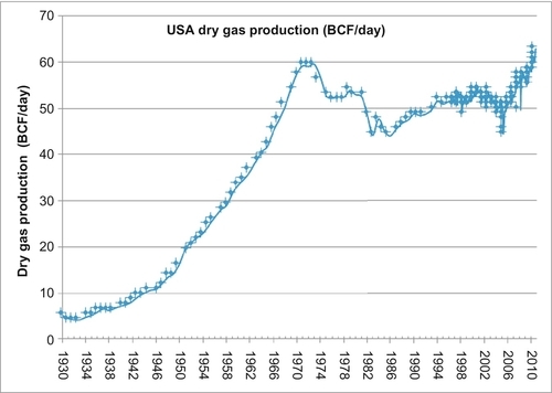
In Figure 5.9, the production rate is shown on an annual basis up until 1997 and on a monthly basis from 1997 until the present time (2011). The decline in production after the peak in 1973, however, did not happen according to Hubbert’s forecast. The rate began to decline for two years then remained constant for five years. The decline then resumes, finally bottoming out at 44 BCF/day in 1986. Since then, there has been a steady increase in production. The production started to increase more sharply in 2006 and today we are making about 68 BCF/day of total gas including 63 BCF/day of dry gas. This is more gas than the United States was making at the peak in 1973. If the production had declined in a mirror image of the front side of the peak, in 2010 the gas production rate should have been the same as in 1936 when the production was only 6 BCF/day. Instead, more than ten times that amount was produced.
The Hubbert method has failed miserably to forecast what has happened on the back side of the curve. The reason for this is economics. Once the nation’s gas supply peaked and a gas shortage developed, the price of gas began to increase. The increased price shook loose gas that was previously uneconomic to produce and people began to develop technologies to find and produce coal-bed methane (also known as coal seam gas), tight gas and shale gas. This type of gas is now known collectively as unconventional gas and it accounts for the majority of the current U.S. gas supply. The United States surpassed Hubbert’s estimate of the total ultimate recovery of 850 trillion cubic feet of gas in 1997, and so far has produced more than 1,120 trillion cubic feet without reaching any new peak. The production is still increasing. Figure 5.10 shows the gas production repeated with the average annual gas price, which illustrates the effect that price has on the supply. The steep increase in the gas price after the peak has created new supplies of gas, causing the Hubbert model to fail on the back side.
The same thing did not happen to the U.S. oil supply curve because the oil market is a global market. The price for U.S. oil could not be pushed up in the same way that the gas price was pushed up because the United States has always imported a significant portion of its oil and so the U.S. oil producers were constrained to the world price of oil. The world price of oil remained relatively low until recently; however, apart from Canadian supplies and a small and expensive Liquefied Natural Gas (LNG) market, the U.S. gas market is relatively insular.
This analogy illustrates that economics affects the supply of commodities such as oil and gas. In the case of the world oil supply, the price of oil has recently been pushed up before the peak of the oil production has been reached. This in turn has pushed out the timing of the peak and indeed the total cumulative production. When the world production of oil does eventually peak (as it must), the back side of the curve will not be a mirror image of the front side of the curve as Hubbert had forecast. It probably will not look like the back side of the U.S. gas supply curve either. It will be controlled by economics and technology, which at this stage are a little difficult to predict.
In his 2010 book When Oil Peaked, Ken Deffeyes presents several proofs and analogies to show that the production curves must be symmetrical, that the back side of the curve must be a mirror image of the front side. All of these proofs depend on a constant oil price, which clearly will not happen. If and when oil production does peak, the shortage of supply will push the price of oil up and the back side of the curve will not be a mirror image of the front side. The fact that the U.S. gas production curve is not symmetrical is an indication of the fallacy of Hubbert’s assumption and the subsequent proofs by Deffeyes. Scenarios can be envisaged where the back side of the world oil production curve might be a mirror image of the front side. At $100/barrel, Gas to Liquids (GTL) technology (see Chapter 6) and Coal to Liquids (CTL) technology (see Chapter 13) is economic. If the world began to shift rapidly to these technologies and they were able to maintain their supply at a high enough rate to keep the price of oil constant, the back side of the oil production curve might then be a mirror image of the front side.
New Supplies of Oil in the United States and the Implications for the World Oil Market
As mentioned earlier, an increase in the world oil price has begun to create new supplies of oil in the United States and this is likely to further increase the world supply. There are a number of areas in North America that are being actively explored, and some of these are likely to contribute significant production to the U.S. oil supply in the immediate future. They include: the Canadian oil sands in Alberta and Saskatchewan; the Bakken formation in North Dakota, Montana, Manitoba and Saskatchewan; the Eagle Ford formation in Texas; the Granite Wash in Oklahoma and the Texas Panhandle; the Niobrara in Colorado and Wyoming; the Monterey in California; the Utica in Ohio; and the Shublik formation on the North Slope of Alaska. The large quantities of oil that have been discovered in the deep waters of the Gulf of Mexico are expected to also play a large role.
Consultants Purvin and Gertz have examined the onshore unconventional oil production from the Bakken, Eagle Ford, and Niobrara plays, and they expect that these three alone will be producing 900,000 b/d by 2015 and exceed 1.3 million b/d by 2020. Currently, oil production from the Bakken and Eagle Ford alone is 350,000-400,000 b/d. These forecasts are pretty conservative. They also leave out the other formations listed above, which will also contribute additional quantities of crude oil and liquid production.
The Bakken formation extends from North Dakota and Montana in the United States to Manitoba and Saskatchewan in Canada (see Figure 5.11). The Bakken is sometimes called the Bakken shale, but the oil production primarily comes from the Middle Bakken zone, which is a low permeability, shale-bearing sandy dolomite. The North Dakota Geological Survey has estimated that there are 250 billion barrels of oil in place in the Bakken and the associated Middle Forks formation just in the North Dakotan part of the play alone. It is not unreasonable to believe that there is an estimated 500 billion barrels of total oil in place in the entire four state/province regions and it is essentially one continuous field. The areas that have been developed there are subdivided into separate fields: the Elm-Coulee in Montana; the Mondak, Parshall, Sanish, Stanley and Ross fields in North Dakota; the Viewfield in Saskatchewan; and the Daly Sinclair in Manitoba. Owing to the low porosity and permeability, the primary recovery is expected to be very low at about 7%. While this number may seem low, 7% of 250 billion barrels is a lot of oil (17.5 billion barrels). When enhanced oil recovery methods such as carbon dioxide miscible flooding are applied, more of the oil can be recovered. This is not proved oil; however, if 17.5 billion barrels were eventually recovered, it would make this the largest oil field ever discovered in North America and one of the largest oil fields in the world.
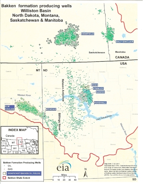
A recent EIA report, released in 2011, estimated that 3.5 billion barrels are recoverable from the U.S. part of the basin. Based on their methodology, this is a very conservative estimate mainly because they have only examined the currently leased acreage. This number changes by using the method of volumetrics to determine the total amount of oil originally in place in the middle Bakken formation. The method is known as volumetrics because you identify the oil in place by calculating the volume that it occupies. This method gives an estimate of original oil in place of 250 billion barrels. The following parameters were used to make this estimate: all of the Bakken area in Figure.5.11 covers more than 35 million acres; the thickness of the Middle Bakken zone is 22 feet; the porosity averages 8% and the oil saturation averages 68%; and the value for the formation volume factor (Bo) is 1.3. The result is 250 billion barrels and this is just the oil in place. To get the recoverable oil, you have to multiply by the recovery factor of 7%, which then gives 17.5 billion barrels of recoverable oil by primary recovery means. The Middle Fork formation, which is below the Bakken formation, will give additional oil, and enhanced oil recovery methods will also increase this number. Even this estimate of 17.5 billion barrels is still relatively low.
In May 2011, the largest operator in the Bakken play—Continental Resources—estimated the primary recoverable reserves in that area to be 24 billion barrels of oil. This was a large increase from previous estimates and was attributed to continuing improvements in drilling and production methods and other technological advances. According to an article in the Oil and Gas Journal (6/6/2011), most operators are drilling 18,000-foot to 21,000-foot wellbores that include 9,500-foot laterals and generally apply 18-30 frac stages per well. Continental based its 24 billion barrel estimate on the following assumptions about two areas of continuous oil reservoirs:
• A recoverable oil volume of 500,000 barrels/well
• Middle Bakken and Three Forks act as separate reservoirs (500,000 barrels/reservoir)
• Dual-zone development (both Middle Bakken and Three Forks reservoirs)
• 320-acre spacing/well (4 wells per zone with 8 wells per 1,280-acre spacing unit)
• Estimated Area 1 having 10,314 square miles (6.6 million acres) in the area where the source rocks are thermally mature, and
• Estimated Area 2 having 4,357 square miles (2.8 million acres) in the area where the source rocks are marginally mature but where mature oil has migrated.
In the article in the Oil and Gas Journal (6/6/2011) Harold Hamm—Continental chairman and chief executive officer—said the industry has completed 3,600 horizontal wells in the Bakken and plans to add 2,100 wells per year using 170-180 drilling rigs that are actively running. Continental restricts initial production rates on many of its North Dakota wells to minimize natural gas flaring and to maximize the volume of rich gas that can be marketed. “Some wells have initial flowing tubing pressures of more than 3,000 psi for several days, so they could easily have tested at double or more their announced rates, if we have opened them up,” Hamm said. As of March 31, Continental had 878,900 net acres leased in the Bakken. As of early May, Continental operated 22 drilling rigs in North Dakota and two in Montana. According to Hamm, six of Continental’s 8 best wells during the first quarter of 2011 were in the Williston prospect where Continental has leased 110,000 net acres.
Type curves for the production from typical Bakken wells are shown in Figure 5.12. The average Bakken well makes about 550,000 barrels ranging from 350,000-700,000 barrels. This number is consistent with Continental’s assumption above. The huge potential of this play is obvious.

To produce oil from the Bakken, the operators have to drill horizontal wells through the formation and then conduct massive fracture stimulation jobs to get the oil to flow out. Oilmen have known about the oil in the Bakken formation since 1950, but they could not produce very much of it at economic rates until these new horizontal drilling and fracture stimulation methods were deployed in the past 5 years. Prior to that, many of the Bakken wells were poor wells, only marginally economic or subeconomic. The new high-tech Bakken wells cost between $5.5 million to $8.5 million to drill and the initial rates are often more than 2,000 barrels per day. Even though these rates decline quickly, at $100 per barrel for the oil, the wells are now very profitable and there is still a lot of oil to be developed there. Activity in the Bakken has pushed North Dakota’s oil production from less than 80,000 barrels per day in 2004 to more than 350,000 barrels per day in 2011. This production will continue to increase. In mid-2011, there were 178 rigs drilling wells in the Bakken play.
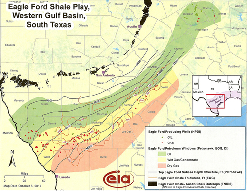
The hottest oil play in the United States in 2011 is the Eagle Ford Shale Play in southwest Texas, which is shown in Figure 5.13. It actually has an oil leg on the northern side of the play, a gas leg on the southern side of the play, with a gas-condensate zone in-between those areas. Gas condensate means that it is a gas phase fluid but there are a lot of liquids volatile in the gas. When the gas is produced, light oil-like liquid called gas condensate drops out of the gas. The gas condensate can be sold as oil, and the gas is sold separately. Due to the fact that oil prices are very high and gas prices are moderately low, the producers derive much more revenue from the oil and condensate production. At the moment, the producers are concentrating on the oil and gas condensate areas of the Eagle Ford play. There is high hope that this area will eventually be producing 500,000 barrels per day of oil and condensate. In mid-2011, there were 195 rigs drilling wells in the Eagle Ford play making it the hottest exploration target in the nation. The EIA estimates of recoveries from the Eagle Ford are 3 billion barrels of oil and 21 trillion cubic feet of gas. Again, these estimates are conservative.
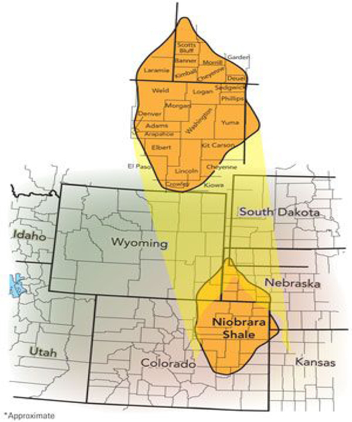
The Niobrara play is barely getting started, but there are high expectations for this play. The area of current interest is in the Denver-Julesberg basin, just north of Denver, Colorado, extending up into Wyoming and over into Nebraska. This is shown in Figure 5.14. The Niobrara formation actually extends beyond this area up into the Powder River Basin in the northeast of Wyoming, and into the Green River basin in the west of Wyoming. If this play proves successful, it is likely to be extended further afield.
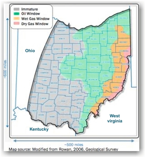
Another recent entry into the shale oil exploration is the Utica shale in eastern Ohio (see Figure 5.15). In late July 2011, Chesapeake Energy Company announced the discovery of a major new liquids-rich play in that area. No estimates of total oil and gas in place or recoverable reserves were made but, based on its geo-scientific, petro-physical and engineering research during the previous two years and the results of six horizontal and nine vertical wells it has drilled, Chesapeake announced that its 1.25 million net leasehold acres in the Utica play could be worth $20 billion in increased value to the company. The company’s dataset on the Utica Shale includes approximately 2,000 well logs on approximately 200 wells, 3,200 feet of core samples from nine wells and production results from three wells. As a result of its analysis, the company believes the Utica Shale will be characterized by a western oil phase, a central wet gas phase and an eastern dry gas phase. It is likely most analogous to the Eagle Ford Shale in South Texas. Chesapeake went so far as to say that it believes that the Utica is economically superior to the Eagle Ford play, and if this proves true, it would make it a very hot exploration target. Chesapeake is currently drilling in the Utica Shale with five rigs to further evaluate and develop its position and anticipates increasing its rig count to eight by the end of 2011 and reaching at least a range of 16-20 rigs by late 2012 and 40 rigs by year-end 2014. Given the 195 rigs currently drilling the Eagle Ford play, this could prove a conservative estimate for the entire play. There will undoubtedly be other such plays in the future that have not been heard of yet.
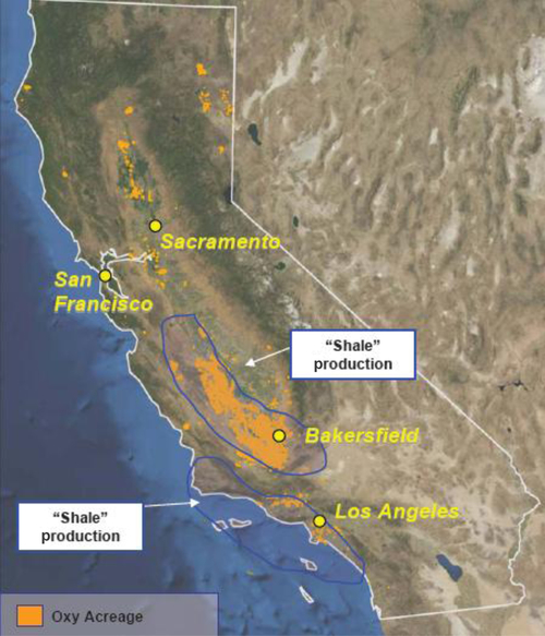
Out in California, there is another shale formation called the Monterey Shale that contains a lot of recoverable oil, and it is also beginning to heat up. The active area for the Monterey shale play is approximately 1,752 square miles in both the San Joaquin and the Los Angeles Basins (see Figure 5.16). The depth of the shale ranges from 8,000 to 14,000 feet deep and is between 1,000 and 3,000 feet thick. The very thickness of the shale in this play allows for a great deal of oil in place. The Monterey is almost pure shale that is naturally fractured in many places. It has been produced through vertical wells for many years, but with the new horizontal drilling and multizone fracture technology, there is increased expectation that much more of the oil can be recovered economically. The recent EIA study has said that there are 15.42 billion barrels of technically recoverable oil in the Monterey shale. Occidental Petroleum (Oxy) has reported that the cost for vertical wells ranges from $2 to $2.5 million and horizontal wells range from $5 to $7 million. They also report that the finding and development costs are between $8 and $18 per barrel depending upon the area of the basin and the quality of the rocks.
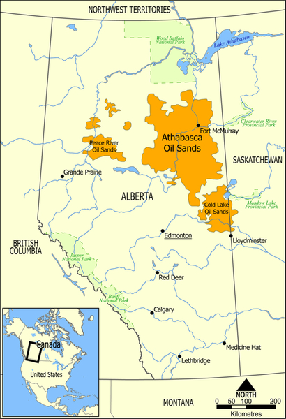
The biggest oil deposits in North America are the oil sand deposits in the Canadian province of Alberta, with some of the deposits extending over into Saskatchewan. Figure 5.17 shows the location of these deposits, which are in three areas: Athabasca, Cold Lake, and Peace River. These deposits consist of very heavy viscous oil that is essentially solid tar. The oil does not flow very well, but the shallowest deposits can be mined by digging up the ground containing the oil and processing it in retorts. They remove the sand grains and add hydrogen to the oil to make it better able to flow through pipes and be refined in refineries. The deeper deposits are contacted through wells where steam is pumped down the well to contact the oil and heat it so that it is less viscous and more able to flow into the well to be produced. This process is known as In-Situ Steam Assisted Gravity Drainage, or SAGD. This technique was developed in the 1980s by the Alberta Oil Sands Technology and Research Authority, but its use depended on the needed improvements in horizontal drilling technology. In SAGD, two horizontal wells are drilled in the oil sands, one at the bottom of the formation and another about 15 feet above it. These wells are typically drilled in groups from a central pad. In each well pair, steam is injected into the upper well and the heat melts the heavy oil, which allows it to flow into the lower well from which it is pumped to the surface. SAGD brings high oil production rates and relatively high recovery factors, sometimes more than 50% of the oil in place.
In a 2011 report entitled Alberta's Energy Reserves 2010 & Supply/Demand Outlook 2011-20, Alberta's Energy Resources Conservation Board (ERCB) noted that the remaining proved oil sands reserves in the Alberta province are 169 billion barrels out of an initial 177 billion barrels of proved reserves. Cumulative oil produced from the oil sands through 2010 has been 7.5 billion barrels since commercial production began. Of the remaining established reserves, mineable areas contain 34 billion barrels and the in situ SAGD areas contain 135 billion bbl. Alberta's production from mining the oil sands in 2010 was 857,000 b/d, which was higher than the 756,000 b/d produced from the in situ areas, but ERCB expects the in situ oil sands production to surpass mining production by 2015. In 2010, all the bitumen produced from mining and 11% of that produced in situ was upgraded in Alberta to yield 795,000 b/d of Synthetic Crude Oil (SCO). ERCB forecast that SCO production in Alberta will increase to 1.4 million b/d by 2020. ERCB also estimates that Alberta holds 1.804 trillion barrels of oil sands initially in place and that the ultimate recovery potential is 315 billion barrels. Compare that to Saudi Arabia’s oil reserves of 263 billion barrels. Alberta's oil sands production is expected to increase to 3.5 million b/d by 2020, up from 1.6 million b/d in 2010. This will make Canada one of the top oil producers in the world.
The entire discussion in this chapter has focused on both the United States and the world’s crude oil production. Currently, the United States uses about 18.5 million b/d of petroleum liquids. This is made up of 6 million b/d of local crude oil production, another 3.5 million b/d of condensate and natural gas liquids (giving 9.5 million b/d of liquids), and 9 million b/d of imported crude oil and petroleum products. Obviously, the condensate and natural gas liquids are contributing significant quantities of liquids to the national supply, which is displacing significant quantities of imported crude oil. This will be important for the future.
The unconventional oil and NGLs that have been reviewed in this section have implications for the future world supply of crude. The technology that is increasing the liquids production in the United States has important implications for world oil supply. The United States is not the only country that has large unconventional resources of oil and gas. As this technology is perfected and the world needs more oil supplies, the methods of production that are being used in the United States will be exported to the rest of the world, which will add to the world supply picture.
The World Picture
The top 20 countries in the world in terms of proved oil reserves are shown in Table 5.1.
Table 5.1
Crude Oil Proved Reserves (Billion Barrels)
| 1 | Saudi Arabia | 262.6 |
| 2 | Venezuela | 211.2 |
| 3 | Canada | 175.2 |
| 4 | Iran | 137.0 |
| 5 | Iraq | 115.0 |
| 6 | Kuwait | 104.0 |
| 7 | United Arab Emirates | 97.8 |
| 8 | Russia | 60.0 |
| 9 | Libya | 46.4 |
| 10 | Nigeria | 37.2 |
| 11 | Kazakhstan | 30.0 |
| 12 | Qatar | 25.4 |
| 13 | United States | 20.7 |
| 14 | China | 20.4 |
| 15 | Brazil | 12.9 |
| 16 | Algeria | 12.2 |
| 17 | Mexico | 10.4 |
| 18 | Angola | 9.5 |
| 19 | Azerbaijan | 7.0 |
| 20 | Ecuador | 6.5 |
Data Source: EIA.
The number two and number three countries on this list, Venezuela and Canada, owe the majority of their reserves to their heavy oil sands. The total reported proved reserves of crude oil for the entire world is 1.3 trillion barrels, although certain peak oil theorists do not believe that these reserves are correct. They believe that some OPEC members inflate their reserves so that they can get a higher production allocation. The fact that OPEC is still restricting their members’ production is evidence that there is spare capacity in the world. If the world’s productive capacity was at 100% or declining, there would no longer be a need for a cartel like OPEC because cartels only exist in order to ration supply in order to keep the price at a certain level. If the members of OPEC were all producing at maximum capacity, they would have no reason to inflate their reserves so that they could get a higher allowable production. On that same note, in May 2011 an influential Saudi Prince—Al-Waleed bin Talal—said that he wants oil prices to drop so that the United States and Europe don’t accelerate efforts to wean themselves off his country’s supply. Prince Al-Waleed is the grandson of the founding king of modern Saudi Arabia (King Saud) and is listed by Forbes as the 26th richest man in the world. He said that the oil price should be somewhere between $70 and $80 a barrel, rather than over $100 a barrel. “We don't want the West to go and find alternatives, because, clearly, the higher the price of oil goes, the more they have incentives to go and find alternatives,” says Prince Al-Waleed. If Saudi Arabia were facing their “twilight in the desert,” a decrease in their productive capacity as claimed by Matthew Simmons, then there would not be a need to take such an attitude. They would be pushing prices as high as possible so that they could maximize their revenue from a declining resource.
The world’s top 30 producing countries are listed in Table 5.2. Production rates should have an approximate correlation to reserves; the higher the reserves, the higher the production rate. In this respect, the United States does very well. It is producing 9.65 million b/d from only 20 billion barrels of reserves. Countries such as Canada and Venezuela clearly have the capacity to increase their production, although most of their reserves are tied up in very heavy oil. This limits their production rates because the viscosity of the oil is so low. If Saudi Arabia really has 263 billion barrels of reserves, they too could increase their rates substantially and they have done this at times. Saudi Arabia, however, has elected to operate as the world’s swing producer, increasing their production when the world demand increases and decreasing production when demand decreases. The Saudis would be happy to increase production if the world demanded it, but they are aware that when the price gets too high, demand decreases and the world starts looking for alternatives. This is why Prince Al-Waleed made the statements that he did. Saudi Arabia would love to sell more oil to the United States and Europe and they have the capacity to do it. Matthew Simmons’ claim in Twilight in the Desert that the oil production of Saudi Arabia has peaked and will soon begin to decline rapidly can only make sense if Saudi Arabia is vastly overstating its reserves. Simmons does try to argue that the Saudis have less oil than they claim but their reserves would have to be about one-tenth of what they claim before they would have trouble keeping up. The United States is producing about the same amount of oil as Saudi Arabia with less than one-tenth of their reserves.
Table 5.2
Crude Oil Production Rates in 2010 (Thousands of Barrels/day)
| 1 | Russia | 9674 |
| 2 | Saudi Arabia | 8900 |
| 3 | United States | 5474 |
| 4 | Iran | 4080 |
| 5 | China | 4076 |
| 6 | Canada | 2734 |
| 7 | Mexico | 2621 |
| 8 | Nigeria | 2455 |
| 9 | United Arab Emirates | 2415 |
| 10 | Iraq | 2399 |
| 11 | Kuwait | 2300 |
| 12 | Venezuela | 2146 |
| 13 | Brazil | 2055 |
| 14 | Angola | 1939 |
| 15 | Norway | 1869 |
| 16 | Algeria | 1729 |
| 17 | Libya | 1650 |
| 18 | Kazakhstan | 1525 |
| 19 | United Kingdom | 1233 |
| 20 | Qatar | 1127 |
| 21 | Azerbaijan | 1035 |
| 22 | Indonesia | 953 |
| 23 | Oman | 865 |
| 24 | Colombia | 786 |
| 25 | India | 751 |
| 26 | Argentina | 642 |
| 27 | Malaysia | 554 |
| 28 | Egypt | 523 |
| 29 | Sudan | 511 |
| 30 | Ecuador | 486 |
Data Source: EIA.
There are other countries that also have the capacity to increase their production, and one way to gauge this is to calculate their reserve life, the number of years it would take to produce their reserves if they keep producing at the current rates. To obtain this number, you divide their reserves (in barrels) by their producing rate (in barrels/year) to get their reserve life in years. Table 5.3 shows the reserve life of the top 30 countries in this category. Any country that has over 30 years of reserve life probably has the potential to increase their production. Number one on the list is Iran. Their production has been somewhat restricted by international sanctions and the lack of access to crucial technology. The United States does not appear in the top 30 on this list because the United States reserve life is only 5.7 years. That is why the catch phrase of “Drill, baby drill” is so apt for the United States. They cannot keep producing oil at its current high rates relative to its reserves unless they are continually drilling new wells and finding more oil. As soon as the United States stops drilling, its production rate plummets and its balance of payment problems gets much worse.
Table 5.3
Reserve Life (Years) of Oil Producing Countries
| 1 | Venezuela | 269.62 |
| 2 | Canada | 175.61 |
| 3 | Iraq | 131.32 |
| 4 | Kuwait | 123.86 |
| 5 | United Arab Emirates | 110.97 |
| 6 | Iran | 91.99 |
| 7 | Saudi Arabia | 80.84 |
| 8 | Libya | 77.08 |
| 9 | Qatar | 61.71 |
| 10 | Kazakhstan | 53.89 |
| 11 | Netherlands | 42.47 |
| 12 | Nigeria | 41.51 |
| 13 | Ecuador | 36.69 |
| 14 | Chad | 32.57 |
| 15 | Yemen | 31.93 |
| 16 | Bolivia | 29.69 |
| 17 | Sudan | 26.79 |
| 18 | Gabon | 24.01 |
| 19 | Egypt | 23.05 |
| 20 | Brunei | 22.13 |
| 21 | Australia | 20.88 |
| 22 | India | 20.72 |
| 23 | Poland | 20.45 |
| 24 | Trinidad and Tobago | 20.31 |
| 25 | Peru | 20.08 |
| 26 | Malaysia | 19.78 |
| 27 | Algeria | 19.34 |
| 28 | Syria | 18.66 |
| 29 | Romania | 18.65 |
| 30 | Azerbaijan | 18.54 |
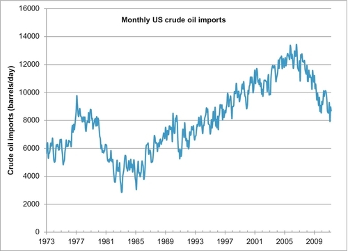
Even though the United States is the third largest oil producer in the world, it is also the largest oil importer in the world and has been so for a long time. Figure 5.18 shows the monthly imports of crude oil into the United States since 1973. There had been a steady increase in imports from 1983, when 4 million b/d were being imported, to August 2006 when 13.4 million b/d were imported. Since then the trend has been back down due to increased production and reduced demand in the United States. In April 2011, only 8.7 million b/d were imported. The United States does have the capacity to reduce this import bill to zero by using its potential for increased production of oil, gas, coal and electricity. This is discussed in more detail in Chapter 16. Even if that goal proves too ambitious, another option would be to reduce its crude imports to 4 million b/d and import all of this from its NAFTA partners, Canada and Mexico. This would make sense if the NAFTA partnership is to be strengthened.
The Future of Oil
The world still has plenty of oil both in production capacity and in future reserves. Any sustained increase in the price of oil will lead to increased reserves and production. The world’s oil production will not peak in the next 10 years. When it does eventually peak, it will not decline rapidly in the manner that the Hubbert Peak Oil Model predicts. The Hubbert bell-shaped production curve is only valid when there is a constant oil price and a constant technology environment; however, price and technology increases also increase the ultimate recoverable reserves, push out the day of reckoning for the peak in oil production and extend the tail of the back side of the curve.